Simulation as a tool for personality research
William Revelle
Northwestern University
To appear in: Personality Research Methods, edited by Robins, Fraley and Krueger
Contents:
- Using the R computer package as a tool for personality research
- Data simulation as a research tool
- Data organization and simple summary statistics
- Using the general linear model to fit data
- Graphical presentations techniques
- Scaling artifacts -- some graphical explorations
Using the R computer package as a tool for personality research
It is useful when learning how to do personality research to consider what ideal results would look like and also to consider the problem of various statistical artifacts. This page, to accompany a chapter on Experimental Approaches to Personality, provides R code for several different simulated studies. For an introduction on how to use R for personality research, consult my notes for personality research. For a somewhat more extensive introduction, try my tutorial for R for Psychological Research.
There are many possible statistical programs that can be used in psychological research. They differ in multiple ways, at least some of which are ease of use, generality, and cost. Some of the more common packages used are Systat, SPSS, and SAS. These programs have GUIs (Graphical User Interfaces) that are relatively easy to use but that are unique to each package. These programs are also very expensive and limited in what they can do. Although convenient to use, GUI based operations are difficult to discuss in written form. When teaching statistics or communicating results to others, it is helpful to use examples that may be used by others using different computing environments and perhaps using different software. The simulations and analyses presented here use an alternative approach that is widely used by practicing statisticians, the statistical environment R. This is not meant as a user's guide to R, but merely a demonstration of the power of R to simulate and analyse personality data. I hope that enough information is provided in this brief guide to make the reader want to learn more. (For the impatient, a brief guide to analyzing data for personality research is also available.)
It has been claimed that "The statistical programming language and computing environment S has become the de-facto standard among statisticians. The S language has two major implementations: the commercial product S-PLUS, and the free, open-source R. Both are available for Windows and Unix/Linux systems; R, in addition, runs on Macintoshes." (From John Fox's short course on S and R).
Data simulation as a research tool
Simulation of data is a surprisingly powerful research tool. For by forcing the theorist to specify the theoretical predictions precisely enough to generate artificial data, theoretical issues are clarified. Parameters need to be specified and relationships need to be identified, not by mere hand waving, but rather by accurate identification. The amount of error in measurement needs to be directly specified in the simulation, requiring the researcher to think about issues of reliability and the shape of latent-observed relationships.
In addition to forcing the theorist to specify the model, by knowing what the right answer is, one can test the power of one's analytical tools to detect the correct model. By knowing the true answer, and observing that small samples do not necessarily detect effects that are there (Type II errors) and that by doing many analyses, the probability of detecting effects that are not there (Type I errors) is higher than expected, the researcher learns greater respect for the problems of good design and good analysis.
By showing the R code for generating simulated data as well as the code for analysis the reader is encouraged to try out some of the techniques for themselves rather than just passively reading yet another chapter.
In all the simulations, data are generated based upon a model that Positive Affect is an interactive and non-linear function of Extraversion and rewarding cues in the environment, that Negative Affect is an additive but non-linear function of Neuroticism and punishing cues in the environment, that arousal is an additive function of stimulant drugs and Introversion, and that cognitive performance is a curvilinear function of arousal. This model is the “truth” that the analyses hope to uncover. Unlike real studies, in all simulations we have access to the latent (but unobserved) “true” variables as well as the observed Person and Outcome variables. (The simulations are based upon somewhat simplified summaries of a number of studies conducted over the past years at the Personality, Motivation and Cognition lab at Northwestern University but are idealizations and simplifications of the actual results of those studies.) Readers are encouraged to try the simulations and analyses for themselves, varying the sample sizes and the strength of the relationships. By presetting the seed for the random number generator to a memorable constant value (Adams, 1980) the results obtained in these simulations and reported below should match those carried out by copying the code in the appendix and running the simulations.
The first section is a simulation of how the personality dimensions of Introversion-Extraversion and Emotional Stability- Neuroticism interact with rewards and punishments to affect Positive and Negative Affect. The simulation uses particular parameter settings that were chosen for pedagogical purposes and only partly reflect published results. For a more detailed discussion of the psychological models being simulated, consult the chapter. For an introduction to personality theory and research, visit the Personality-Project.
The second simulation models the interactive effect on cognitive performance of the personality variable introversion-extraversion with arousal inductions such as caffeine. This is also based upon work at the Personality, Motivation and Cognition lab.
The third simulation is concerned with problems of scaling and shows how it important it is to choose the appropriate metric.
All simulations make use of some useful additions to R that may be found in the "psych" package at the personality-project.org. To use these additions, first load R and then use the package manager and installer.
Simulation 1: Personality and Rewards and Punishments
The following code is directly executable in R. The user is encouraged to modify the parameters to explore further how to detect main effects and interactions in personality research. The text in blue is directly executable and should be copied into R. Results and graphics from these commands are included for comparison purposes.
Note: To reproduce the same "random" simulations each time, include the set.seed(42) command. To make a different simulation each time, do not include that line.
#R code for simulating personality x situation effects
#
#Part 1: Simulate the data

set.seed(42)   #random number seed is fixed to produce identical "random" sequences
               #remove to allow each run to be different

#first set some parameters of the model
#change these to try different models

num <- 100    		#number of people to simulate
weightreward <- .5 #an index of how strong is the effect of reward on positive affect
weightpunish <- .4  #how strong is the effect of punishment on negative affect
weight_e<-  .0 		#how strong is the effect of extraversion on positive affect
weight_n<-  .3 		#how strong is the effect of neuroticism on negative affect?
weight_er <-.4 		#how strong is the interaction of e x reward on positive affect
weight_np <- 0 		#how strong is the interactionof n * punish on negative affect
reliability_e <- .7	#the reliability of the observed extraversion score
reliability_n <-.8   #the reliability of the observed neuroticism score
reliability_P <-.7   #the reliability of observed measures of Postive Affect
reliability_N <- .8  #the reliability of observed measures of Negative Affect
weight_arousal <- .7	#relationship between extraversion and arousal
reliability_arousal <- .8 #reliability of arousal
weight_caff <- .5    #within subject weight of effect of caffeine
mean_E <- 3 		#mean of true extraversion
mean_N <- 3			#mean of true neuroticism

#generate the data using the random normal distribution

						#first simulate true (latent) scores
true_e <- rnorm(num,mean_E)   #true trait extraversion is normally distributed with sigma=1
true_n <- rnorm(num,mean_N)   	#true trait neuroticism is normally distributed
true_arousal_plac <- rnorm(num) - weight_arousal * (true_e - mean_E) -weight_caff
true_arousal_caff <- rnorm(num) - weight_arousal * (true_e - mean_E) + weight_caff
                        #observed E and N are a mixture of true and error scores
extraversion <- sqrt(reliability_e)*(true_e-mean_E) + sqrt(1-reliability_e)*rnorm(num) + mean_E
neuroticism <- sqrt(reliability_n)*(true_n -mean_N)+ sqrt(1-reliability_n)*rnorm(num) + mean_N
arousal_plac <- sqrt(reliability_arousal) * (true_arousal_plac) + sqrt(1-reliability_arousal)*rnorm(num)
arousal_caff <- sqrt(reliability_arousal) * (true_arousal_caff) + sqrt(1-reliability_arousal)*rnorm(num)
performance_plac <- (1/(1+exp(-true_arousal_plac)))*(1/(1+exp(true_arousal_plac)))   #inverted u function of arousal
performance_caff <- (1/(1+exp(-true_arousal_caff)))*(1/(1+exp(true_arousal_caff)))   #inverted u function of arousal

						#experimental conditions are block randomized
reward <- rep(c(0,1),num/2)   #reward vector of 0 or 1
punish <- rep(c(0,0,1,1),num/4) #punishment vector
block <- sort(rep(seq(1:(num/4)),4))  #block the data to allow for block randomization
temp.condition <- data.frame(reward,punish,block,rand =rnorm(num))  #experimental conditions ordered by block
condition <- temp.condition[order(temp.condition$block,temp.condition$rand),1:2]  #conditions are now block randomized


#true affect measures are a function of a trait, a situation, and their interaction
TruePosAffect <- 1/(1+exp(-(weight_e * true_e + weightreward * condition$reward +weight_er * true_e * condition$reward)))
TrueNegAffect <- 1/(1+exp(-(weight_n * true_n + weightpunish * condition$punish +weight_np * true_n * condition$punish )))
TruePosAffect <- scale(TruePosAffect)     #standardize TruePosAffect to put on the same metric as the error scores
TrueNegAffect <- scale(TrueNegAffect)     #standardize TrueNegAffect to put on the same metric as the error scores

#observed affect is a function of true affect and errors in measurement
PosAffect <- sqrt(reliability_P) * TruePosAffect+sqrt(1-reliability_P)*rnorm(num)
NegAffect <- sqrt(reliability_N) * TrueNegAffect+sqrt(1-reliability_N)*rnorm(num)
Data Organization
The data have been simulated and are ready for analysis. When doing the following analyses it is simpler if the data are organized in "data.frames" which are analogous to matrices except that different types of variables can be in different columns.
The analyses will be done as moderated multiple regression. This requires certain modifications to the data before putting them into a data frame. The most important is to center the Person Variable predictors around their mean and to convert the Experimental Variables to "factors" or categorical variables. The centering operation makes the product terms independent of the main effects.
In addition, some of the data should be transformed to allow for alernative demonstrations of analytic techniques. One transform is merely finding the sums and differences of the affect measures. This will be useful when we show that mixed within-between subject ANOVA can be thought of as a combination of two separate ANOVAS, one between subjects and one within subjects.
#organize all the data in a data frame to allow for analysis
#because it is also possible to do repeated measures as ANOVA on sums and differences
#the between effects are found by the sums
#the within effects are found the differences

PosplusNeg = PosAffect+NegAffect
PosminusNeg <- PosAffect - NegAffect
affect.data <- data.frame(extraversion,neuroticism,PosAffect,NegAffect,PosplusNeg,PosminusNeg,true_e,true_n,TruePosAffect,TrueNegAffect,
reward = as.factor(condition$reward),punish=as.factor(condition$punish))
centered.affect.data <- data.frame(scale(affect.data[,1:10],scale=FALSE),reward = as.factor(condition$reward),punish=as.factor(condition$punish))
drug.data <- data.frame(extraversion,true_arousal_plac,true_arousal_caff,arousal_plac,arousal_caff,performance_plac,performance_caff)


rm(reward,punish,block,condition,TruePosAffect,TrueNegAffect,PosAffect,NegAffect,extraversion, neuroticism, true_e, true_n,PosplusNeg,PosminusNeg,
true_arousal_plac,true_arousal_caff,arousal_plac,arousal_caff,performance_plac,performance_caff)
    #these have all been put into  data.frames and we don't need them individually anymore
The artificial data sets have been simulated and stored into three "data.frames" for easier manipulation. We can show the first 5 lines of the data.frame:
 print(affect.data[1:5,],digits=2)
  extraversion neuroticism PosAffect NegAffect PosplusNeg PosminusNeg true_e true_n TruePosAffect TrueNegAffect reward punish
1          4.9         4.5      1.63      2.45       4.08       -0.83    4.4    4.2          1.33           1.6      1      1
2          2.1         4.3     -0.95      1.56       0.61       -2.50    2.4    4.0         -0.97           1.5      0      1
3          3.3         2.1     -0.76     -0.91      -1.67        0.15    3.4    2.0         -0.97          -1.5      0      0
4          3.6         4.7      0.74      1.16       1.90       -0.43    3.6    4.8          1.17           1.1      1      0
5          3.0         2.1      0.38     -1.47      -1.09        1.85    3.4    2.3         -0.97          -1.1      0      0
The centered data have had the means removed:
 print(centered.affect.data[1:5,],digits=2)
  extraversion neuroticism PosAffect NegAffect PosplusNeg PosminusNeg true_e true_n TruePosAffect TrueNegAffect reward punish
1        1.916        1.61      1.58      2.51       4.09       -0.93   1.34   1.29          1.33           1.6      1      1
2       -0.911        1.42     -0.99      1.61       0.62       -2.61  -0.60   1.13         -0.97           1.5      0      1
3        0.372       -0.82     -0.80     -0.85      -1.66        0.05   0.33  -0.92         -0.97          -1.5      0      0
4        0.594        1.79      0.69      1.22       1.91       -0.53   0.60   1.94          1.17           1.1      1      0
5        0.059       -0.84      0.34     -1.41      -1.08        1.75   0.37  -0.58         -0.97          -1.1      0      0
>
Basic descriptive statistics (using describe)
Basic descriptive statistics can be found by using the summary (), describe() and pairs.panels functions. (Describe and pairs.panels are part of the "psych" package.)
describe(affect.data)
              var   n  mean   sd median   min  max range   se
extraversion    1 100  2.96 1.07   3.05  0.33 5.50  5.16 0.11
neuroticism     2 100  2.92 0.85   2.88  0.92 5.26  4.34 0.09
PosAffect       3 100  0.05 1.09  -0.03 -2.43 2.70  5.13 0.11
NegAffect       4 100 -0.06 0.98   0.05 -2.11 2.45  4.56 0.10
PosplusNeg      5 100 -0.01 1.48   0.12 -2.73 4.08  6.81 0.15
PosminusNeg     6 100  0.10 1.46   0.04 -3.24 3.13  6.37 0.15
true_e          7 100  3.03 1.04   3.09  0.01 5.29  5.28 0.10
true_n          8 100  2.91 0.90   2.93  0.98 5.70  4.73 0.09
TruePosAffect   9 100  0.00 1.00  -0.48 -0.97 1.48  2.45 0.10
TrueNegAffect  10 100  0.00 1.00   0.26 -2.66 1.95  4.60 0.10
reward         11  NA    NA 0.50     NA    NA   NA    NA   NA
punish         12  NA    NA 0.50     NA    NA   NA    NA   NA


describe(drug.data)


                  var   n  mean   sd median   min  max range   se
extraversion        1 100  2.96 1.07   3.05  0.33 5.50  5.16 0.11
true_arousal_plac   2 100 -0.53 1.33  -0.45 -3.84 2.84  6.68 0.13
true_arousal_caff   3 100  0.51 1.10   0.51 -2.19 3.06  5.25 0.11
arousal_plac        4 100 -0.52 1.28  -0.43 -4.11 2.96  7.08 0.13
arousal_caff        5 100  0.38 1.04   0.36 -2.09 3.25  5.33 0.10
performance_plac    6 100  0.18 0.07   0.21  0.02 0.25  0.23 0.01
performance_caff    7 100  0.19 0.06   0.21  0.04 0.25  0.21 0.01
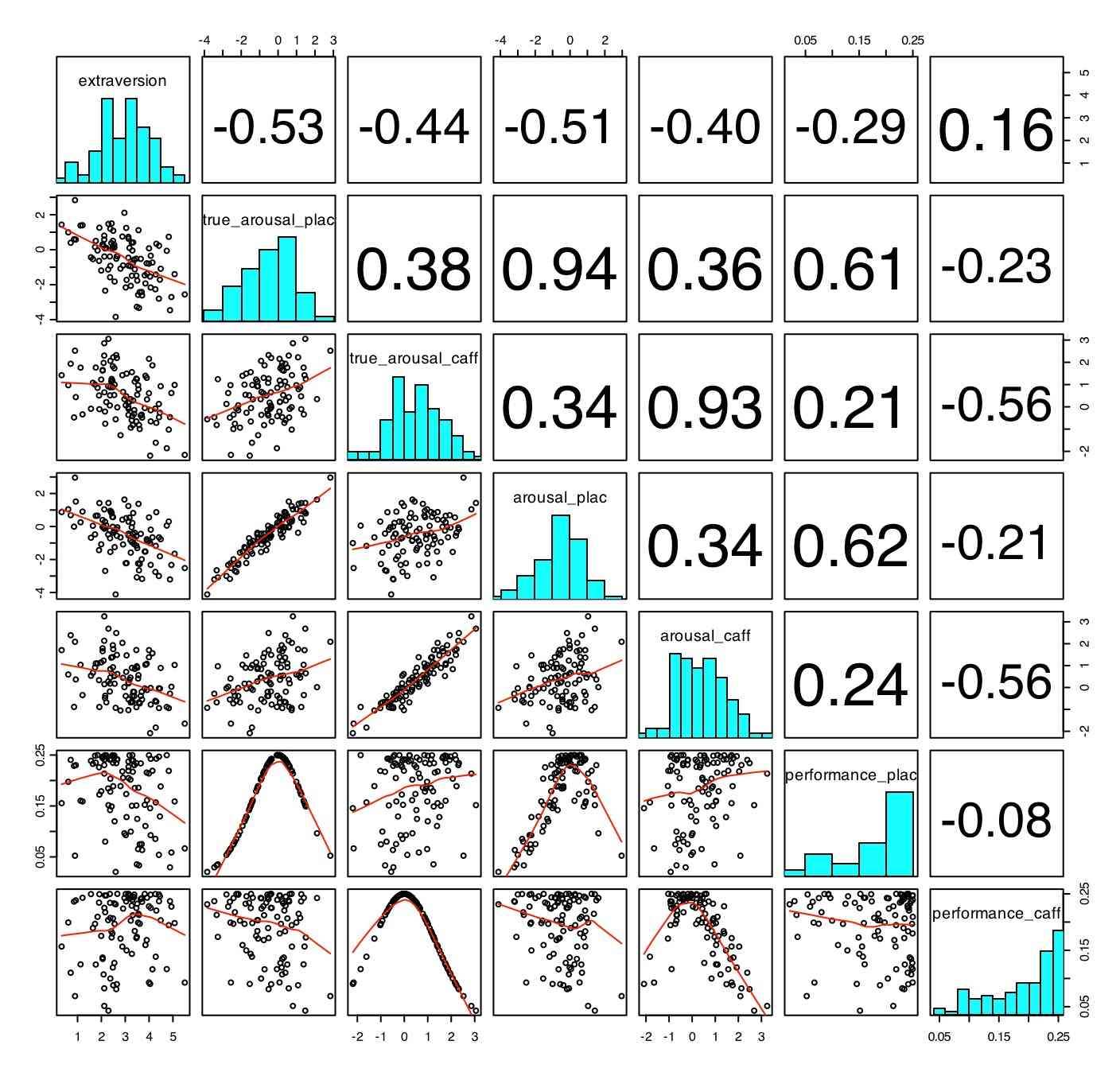
Basic descriptive statistics -- graphical presentation (using pairs.panels)
The data can also be visualized using the pairs.panels function (adapted from the pairs function of base R).
Part 3: Analyse the data using ANOVA and the general linear model.
Some of the analyses are shown merely to allow the user to appreciate the differences between various ways of model fitting.
#the first models do not use 0 centered data and are incorrect
#these are included merely to show what happens if the correct model is not used
#do the analyses using  a linear model without centering the data   ---- wrong
mod1w <- lm(PosAffect ~ extraversion+reward,data= affect.data)   #don't exam interactions
mod2w <- lm(NegAffect ~ neuroticism+punish,data = affect.data)
mod3w <- lm(PosAffect ~ extraversion*reward,data = affect.data) #look for interactions
mod4w <- lm(NegAffect ~ neuroticism*punish,data = affect.data)
mod5w <- lm(PosAffect ~ extraversion*neuroticism*reward*punish,data = affect.data)
				#show the results of the analyses
summary(mod1w,digits=2)
summary(mod2w,digits=2)
summary(mod3w,digits=2)
summary(mod4w,digits=2)
summary(mod5w,digits=2)


#do the analyses with centered data   -- this is the correct way -- note the differences
#just look at main effects
mod1 <- lm(NegAffect ~ neuroticism+punish,data = centered.affect.data)   #just main effects
mod2 <- lm(PosAffect ~ extraversion+reward,data= centered.affect.data)   #don't exam interactions

#include interactions
# note that mod3 and mod4 are two different ways of specifying the interaction
mod3 <- lm(PosAffect ~ extraversion*reward,data = centered.affect.data) #look for interactions
mod4 <- lm(NegAffect ~ neuroticism+ punish + neuroticism*punish,data = centered.affect.data)
#go for the full models
mod5 <- lm(PosAffect ~ extraversion*neuroticism*reward*punish,data = centered.affect.data)
mod6 <- lm(NegAffect ~ extraversion*neuroticism*reward*punish,data = centered.affect.data)
mod6.5  <- lm(c(NegAffect,PosAffect) ~ extraversion*neuroticism*reward*punish,data = centered.affect.data)


				#show the results of the analyses
summary(mod1,digits=2)
summary(mod2,digits=2)
summary(mod3,digits=2)
summary(mod4,digits=2)
summary(mod5,digits=2)
summary(mod6,digits=2)
Produces the following output
The first two analyses are just looking for main effects and are not as interesting as the third one.
 summary(mod1,digits=2)   #just the main effects of neuroticism and the negative film

Call:
lm(formula = NegAffect ~ neuroticism + punish, data = centered.affect.data)

Residuals:
      Min        1Q    Median        3Q       Max
-1.570842 -0.313535  0.004136  0.329371  1.269003

Coefficients:
            Estimate Std. Error t value Pr(>|t|)
(Intercept) -0.54682    0.07814  -6.998 3.37e-10 ***
neuroticism  0.72367    0.06514  11.110  < 2e-16 ***
punish1      1.09364    0.11053   9.895 2.26e-16 ***
---
Signif. codes:  0 ‘***’ 0.001 ‘**’ 0.01 ‘*’ 0.05 ‘.’ 0.1 ‘ ’ 1

Residual standard error: 0.5524 on 97 degrees of freedom
Multiple R-Squared: 0.6891,	Adjusted R-squared: 0.6827
F-statistic: 107.5 on 2 and 97 DF,  p-value: < 2.2e-16

> summary(mod2,digits=2)   #just extraversion + rewarding film

Call:
lm(formula = PosAffect ~ extraversion + reward, data = centered.affect.data)

Residuals:
     Min       1Q   Median       3Q      Max
-2.13532 -0.46240  0.09547  0.43269  1.93528

Coefficients:
             Estimate Std. Error t value Pr(>|t|)
(Intercept)  -0.84505    0.09716  -8.697 8.67e-14 ***
extraversion  0.13151    0.06432   2.045   0.0436 *
reward1       1.69010    0.13745  12.296  < 2e-16 ***
---
Signif. codes:  0 ‘***’ 0.001 ‘**’ 0.01 ‘*’ 0.05 ‘.’ 0.1 ‘ ’ 1

Residual standard error: 0.6869 on 97 degrees of freedom
Multiple R-Squared: 0.6133,	Adjusted R-squared: 0.6054
F-statistic: 76.93 on 2 and 97 DF,  p-value: < 2.2e-16

> summary(mod3,digits=2)   #this one includes the interaction, compare it to model 2

Call:
lm(formula = PosAffect ~ extraversion * reward, data = centered.affect.data)

Residuals:
    Min      1Q  Median      3Q     Max
-2.0622 -0.4644  0.0832  0.4447  2.0437

Coefficients:
                      Estimate Std. Error t value Pr(>|t|)
(Intercept)          -0.840116   0.095747  -8.774 6.37e-14 ***
extraversion         -0.005329   0.093516  -0.057   0.9547
reward1               1.689352   0.135401  12.477  < 2e-16 ***
extraversion:reward1  0.252946   0.127146   1.989   0.0495 *
---
Signif. codes:  0 ‘***’ 0.001 ‘**’ 0.01 ‘*’ 0.05 ‘.’ 0.1 ‘ ’ 1

Residual standard error: 0.6766 on 96 degrees of freedom
Multiple R-Squared: 0.6286,	Adjusted R-squared: 0.617
F-statistic: 54.17 on 3 and 96 DF,  p-value: < 2.2e-16

> summary(mod4,digits=2)   # the interaction is not significant -- compare to model 1

Call:
lm(formula = NegAffect ~ neuroticism + punish + neuroticism *
    punish, data = centered.affect.data)

Residuals:
      Min        1Q    Median        3Q       Max
-1.565723 -0.309362  0.003068  0.330083  1.264219

Coefficients:
                    Estimate Std. Error t value Pr(>|t|)
(Intercept)         -0.54665    0.07855  -6.959 4.21e-10 ***
neuroticism          0.71679    0.08752   8.190 1.12e-12 ***
punish1              1.09369    0.11110   9.845 3.21e-16 ***
neuroticism:punish1  0.01561    0.13188   0.118    0.906
---
Signif. codes:  0 ‘***’ 0.001 ‘**’ 0.01 ‘*’ 0.05 ‘.’ 0.1 ‘ ’ 1

Residual standard error: 0.5552 on 96 degrees of freedom
Multiple R-Squared: 0.6892,	Adjusted R-squared: 0.6795
F-statistic: 70.95 on 3 and 96 DF,  p-value: < 2.2e-16
We can see this relationship more clearly if we graph it. In this plot, we show both the "true" data as well as the observed data. Plotting commands for this are given in the graphics section.
Figure 1: The effect of negative feedback or a sad movie upon Negative Affect
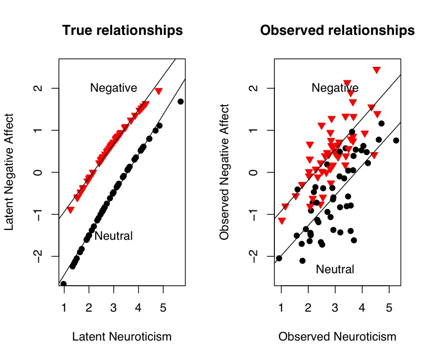
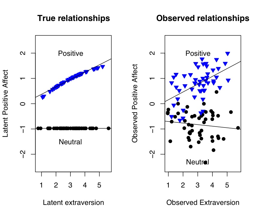
Figure 2: The effect of positive feedback or a happy movie upon Positive Affect
> summary(mod5,digits=2)

Call:
lm(formula = PosAffect ~ extraversion * neuroticism * reward *
    punish, data = centered.affect.data)

Residuals:
     Min       1Q   Median       3Q      Max
-2.12045 -0.41413  0.07548  0.48669  2.00568

Coefficients:
                                         Estimate Std. Error t value Pr(>|t|)
(Intercept)                              -0.63697    0.14799  -4.304 4.51e-05 ***
extraversion                              0.07457    0.14006   0.532   0.5958
neuroticism                              -0.04179    0.17649  -0.237   0.8134
reward1                                   1.45328    0.20803   6.986 6.20e-10 ***
punish1                                  -0.42974    0.20259  -2.121   0.0369 *
extraversion:neuroticism                 -0.04462    0.12356  -0.361   0.7189
extraversion:reward1                      0.09537    0.20149   0.473   0.6372
neuroticism:reward1                      -0.03706    0.23454  -0.158   0.8748
extraversion:punish1                     -0.24191    0.21731  -1.113   0.2688
neuroticism:punish1                       0.05500    0.28466   0.193   0.8473
reward1:punish1                           0.44668    0.29069   1.537   0.1281
extraversion:neuroticism:reward1         -0.19181    0.21128  -0.908   0.3666
extraversion:neuroticism:punish1         -0.03263    0.29695  -0.110   0.9128
extraversion:reward1:punish1              0.39800    0.28834   1.380   0.1711
neuroticism:reward1:punish1              -0.12139    0.36464  -0.333   0.7400
extraversion:neuroticism:reward1:punish1  0.27421    0.36118   0.759   0.4498
---
Signif. codes:  0 ‘***’ 0.001 ‘**’ 0.01 ‘*’ 0.05 ‘.’ 0.1 ‘ ’ 1

Residual standard error: 0.6821 on 84 degrees of freedom
Multiple R-Squared: 0.6698,	Adjusted R-squared: 0.6108
F-statistic: 11.36 on 15 and 84 DF,  p-value: 1.618e-14

> summary(mod6,digits=2)

Call:
lm(formula = NegAffect ~ extraversion * neuroticism * reward *
    punish, data = centered.affect.data)

Residuals:
     Min       1Q   Median       3Q      Max
-1.14498 -0.33986  0.01124  0.34204  1.20472

Coefficients:
                                         Estimate Std. Error t value Pr(>|t|)
(Intercept)                              -0.75119    0.11463  -6.553 4.29e-09 ***
extraversion                              0.24492    0.10848   2.258  0.02656 *
neuroticism                               0.79015    0.13670   5.780 1.23e-07 ***
reward1                                   0.44853    0.16113   2.784  0.00664 **
punish1                                   1.33237    0.15692   8.491 6.28e-13 ***
extraversion:neuroticism                  0.02834    0.09570   0.296  0.76787
extraversion:reward1                     -0.16061    0.15606  -1.029  0.30638
neuroticism:reward1                      -0.04336    0.18167  -0.239  0.81193
extraversion:punish1                     -0.39715    0.16832  -2.360  0.02062 *
neuroticism:punish1                      -0.04101    0.22048  -0.186  0.85290
reward1:punish1                          -0.48703    0.22516  -2.163  0.03338 *
extraversion:neuroticism:reward1         -0.27373    0.16365  -1.673  0.09811 .
extraversion:neuroticism:punish1          0.06403    0.23000   0.278  0.78138
extraversion:reward1:punish1              0.18717    0.22333   0.838  0.40437
neuroticism:reward1:punish1               0.07575    0.28244   0.268  0.78919
extraversion:neuroticism:reward1:punish1  0.20111    0.27975   0.719  0.47420
---
Signif. codes:  0 ‘***’ 0.001 ‘**’ 0.01 ‘*’ 0.05 ‘.’ 0.1 ‘ ’ 1

Residual standard error: 0.5283 on 84 degrees of freedom
Multiple R-Squared: 0.7538,	Adjusted R-squared: 0.7098
F-statistic: 17.14 on 15 and 84 DF,  p-value: < 2.2e-16
Note that the last two analyses could have been done in parallel by combining them into one model:
mod6.5  <- lm(c(NegAffect,PosAffect) ~ extraversion*neuroticism*reward*punish,data = centered.affect.data)
summary(mod6.5)
Multiple Dependent Measures- MANOVA
In the case of multiple dependent measures, there are a number of ways to treat the data. Multivariate Analysis of Variance (MANOVA) exams whether the various predictor variables have an overall effect upon all the dependent variables. If they do, then one can proceed to examine the separate dependent variables.
Traditionally, when examining several dependent variables (e.g., positive and negative affect), one might be interested in whether there is a difference in the effects depending upon which dependent variable is examined. That is, is there an interaction of dependent variable by some treatment?
#try MANOVA


mfit <- manova(cbind(PosAffect,NegAffect)~extraversion*neuroticism*reward*punish,data=centered.affect.data)
summary(mfit)
summary.aov(mfit)    #gives the "simple fits" for both dependent variables
The Manova output gives an overall test of the model, as well as separate estimates for each of the dependent variables:
mfit <- manova(cbind(PosAffect,NegAffect)~extraversion*neuroticism*reward*punish,data=centered.affect.data)
> summary(mfit)
                                       Df Pillai approx F num Df den Df    Pr(>F)
extraversion                            1  0.037    1.612      2     83   0.20561
neuroticism                             1  0.623   68.525      2     83 < 2.2e-16 ***
reward                                  1  0.644   75.235      2     83 < 2.2e-16 ***
punish                                  1  0.577   56.633      2     83 3.081e-16 ***
extraversion:neuroticism                1  0.012    0.525      2     83   0.59339
extraversion:reward                     1  0.090    4.123      2     83   0.01963 *
neuroticism:reward                      1  0.009    0.372      2     83   0.69070
extraversion:punish                     1  0.084    3.801      2     83   0.02633 *
neuroticism:punish                      1  0.001    0.022      2     83   0.97834
reward:punish                           1  0.099    4.538      2     83   0.01348 *
extraversion:neuroticism:reward         1  0.013    0.529      2     83   0.59089
extraversion:neuroticism:punish         1  0.038    1.634      2     83   0.20141
extraversion:reward:punish              1  0.023    0.961      2     83   0.38663
neuroticism:reward:punish               1  0.004    0.152      2     83   0.85887
extraversion:neuroticism:reward:punish  1  0.011    0.461      2     83   0.63195
Residuals                              84
---
Signif. codes:  0 ‘***’ 0.001 ‘**’ 0.01 ‘*’ 0.05 ‘.’ 0.1 ‘ ’ 1
> summary.aov(mfit)    #gives the "simple fits" for both dependent variables
 Response PosAffect :
                                       Df    Sum Sq   Mean Sq   F value  Pr(>F)
extraversion                            1     1.254     1.254    2.6965 0.10431
neuroticism                             1     0.718     0.718    1.5442 0.21746
reward                                  1    70.663    70.663  151.8904 < 2e-16 ***
punish                                  1     0.659     0.659    1.4165 0.23733
extraversion:neuroticism                1     0.342     0.342    0.7347 0.39381
extraversion:reward                     1     2.531     2.531    5.4404 0.02207 *
neuroticism:reward                      1     0.012     0.012    0.0263 0.87151
extraversion:punish                     1     0.059     0.059    0.1270 0.72244
neuroticism:punish                      1 5.367e-08 5.367e-08 1.154e-07 0.99973
reward:punish                           1     1.321     1.321    2.8399 0.09566 .
extraversion:neuroticism:reward         1     0.069     0.069    0.1486 0.70090
extraversion:neuroticism:punish         1     0.465     0.465    0.9997 0.32024
extraversion:reward:punish              1     0.779     0.779    1.6752 0.19912
neuroticism:reward:punish               1     0.125     0.125    0.2687 0.60558
extraversion:neuroticism:reward:punish  1     0.268     0.268    0.5764 0.44985
Residuals                              84    39.079     0.465
---
Signif. codes:  0 ‘***’ 0.001 ‘**’ 0.01 ‘*’ 0.05 ‘.’ 0.1 ‘ ’ 1

 Response NegAffect :
                                       Df Sum Sq Mean Sq  F value    Pr(>F)
extraversion                            1  0.292   0.292   1.0449  0.309626
neuroticism                             1 35.812  35.812 128.3103 < 2.2e-16 ***
reward                                  1  0.616   0.616   2.2080  0.141039
punish                                  1 29.501  29.501 105.6980 < 2.2e-16 ***
extraversion:neuroticism                1  0.049   0.049   0.1750  0.676764
extraversion:reward                     1  0.458   0.458   1.6413  0.203671
neuroticism:reward                      1  0.184   0.184   0.6591  0.419156
extraversion:punish                     1  2.144   2.144   7.6801  0.006874 **
neuroticism:punish                      1  0.012   0.012   0.0430  0.836194
reward:punish                           1  1.344   1.344   4.8154  0.030968 *
extraversion:neuroticism:reward         1  0.286   0.286   1.0251  0.314211
extraversion:neuroticism:punish         1  0.776   0.776   2.7799  0.099181 .
extraversion:reward:punish              1  0.150   0.150   0.5378  0.465375
neuroticism:reward:punish               1  0.003   0.003   0.0117  0.914114
extraversion:neuroticism:reward:punish  1  0.144   0.144   0.5168  0.474199
Residuals                              84 23.445   0.279
---
Signif. codes:  0 ‘***’ 0.001 ‘**’ 0.01 ‘*’ 0.05 ‘.’ 0.1 ‘ ’ 1
Multiple Dependent Measures- Repeated Measures
Traditionally, when examining several dependent variables (e.g., positive and negative affect), one might be interested in whether there is a difference in the effects depending upon which dependent variable is examined. That is, is there an interaction of dependent variable by some treatment? Until recently this has led to the use of repeated measures analysis of variance. The first two examples (models 7 and 8) demonstrate that the repeated measures can be broken up into two separate analyses, one looking at the sums of the scores, one looking at the differences of the scores. Compare these two to the repeated measures model (mod9). Although the Sums of Squares differ for the two models, note how the Mean Squares, F values, and resulting P values are identical for these two ways of thinking about the data.
#models 7 and 8 are included to show how there are alternative ways of doing a within subjects analysis
mod7 <- lm(PosplusNeg  ~ extraversion*neuroticism*reward*punish,data = centered.affect.data)    # this does the equivalent of the between part of a within-between analysis
mod8 <- lm(PosminusNeg  ~ extraversion*neuroticism*reward*punish,data = centered.affect.data)    # this does the equivalent of the within part of a within-between analysis

summary(mod7,digits=2)
summary(mod8,digits=2)

#repeated measures ANOVA
#this requires a bit more work, in that we need to string out the data
attach(centered.affect.data)

PosNeg.df <- data.frame(PosAffect,NegAffect)   #make this into a 2 column data frame
stacked.pn <- stack(PosNeg.df)                 #string the data out for analysis
design.df <- data.frame(stacked.pn,rbind(centered.affect.data,centered.affect.data),subj=gl(num,1,2*num))
#note that subject is a factor in the repeated measures design
#the gl() function creates the factors
#design.df        #show the data frame to understand it
detach(centered.affect.data)


mod7 <- aov(values ~ ind*extraversion*neuroticism*reward*punish+Error(subj),data=design.df)
summary(mod7)

#also possible to do repeated measures as ANOVA on sums and differences
#the between effects are found by the sums
#the within effects are found the differences
#thus, the following two analyses are the same as model 7
mod8 <- aov(PosplusNeg ~extraversion*neuroticism*reward*punish,data=centered.affect.data)
#
mod9 <- aov(PosminusNeg ~extraversion*neuroticism*reward*punish,data=centered.affect.data)
summary(mod8)    #the between part of model 7
summary(mod9)    #the within part of model 7
These analyses produce the following output:
summary(mod7)

Error: subj
                                       Df    Sum Sq   Mean Sq F value    Pr(>F)
extraversion                            1     1.378     1.378  3.1773   0.07828 .
neuroticism                             1    13.193    13.193 30.4219 3.763e-07 ***
reward                                  1    42.239    42.239 97.3986 1.063e-15 ***
punish                                  1    10.671    10.671 24.6055 3.623e-06 ***
extraversion:neuroticism                1     0.066     0.066  0.1524   0.69720
extraversion:reward                     1     0.418     0.418  0.9633   0.32916
neuroticism:reward                      1     0.051     0.051  0.1168   0.73341
extraversion:punish                     1     1.457     1.457  3.3602   0.07033 .
neuroticism:punish                      1     0.006     0.006  0.0138   0.90682
reward:punish                           1 4.866e-05 4.866e-05  0.0001   0.99157
extraversion:neuroticism:reward         1     0.318     0.318  0.7338   0.39408
extraversion:neuroticism:punish         1     1.221     1.221  2.8160   0.09705 .
extraversion:reward:punish              1     0.807     0.807  1.8603   0.17624
neuroticism:reward:punish               1     0.044     0.044  0.1013   0.75108
extraversion:neuroticism:reward:punish  1     0.403     0.403  0.9290   0.33789
Residuals                              84    36.428     0.434
---
Signif. codes:  0 ‘***’ 0.001 ‘**’ 0.01 ‘*’ 0.05 ‘.’ 0.1 ‘ ’ 1

Error: Within
                                           Df    Sum Sq   Mean Sq   F value    Pr(>F)
ind                                         1 3.755e-31 3.755e-31 1.209e-30  1.000000
ind:extraversion                            1    0.1682    0.1682    0.5415  0.463880
ind:neuroticism                             1   23.3372   23.3372   75.1217 2.774e-13 ***
ind:reward                                  1   29.0406   29.0406   93.4806 2.683e-15 ***
ind:punish                                  1   19.4891   19.4891   62.7346 8.747e-12 ***
ind:extraversion:neuroticism                1    0.3245    0.3245    1.0446  0.309678
ind:extraversion:reward                     1    2.5713    2.5713    8.2770  0.005089 **
ind:neuroticism:reward                      1    0.1456    0.1456    0.4686  0.495521
ind:extraversion:punish                     1    0.7454    0.7454    2.3995  0.125136
ind:neuroticism:punish                      1    0.0060    0.0060    0.0194  0.889542
ind:reward:punish                           1    2.6651    2.6651    8.5790  0.004377 **
ind:extraversion:neuroticism:reward         1    0.0370    0.0370    0.1191  0.730890
ind:extraversion:neuroticism:punish         1    0.0198    0.0198    0.0636  0.801448
ind:extraversion:reward:punish              1    0.1227    0.1227    0.3949  0.531428
ind:neuroticism:reward:punish               1    0.0843    0.0843    0.2715  0.603714
ind:extraversion:neuroticism:reward:punish  1    0.0095    0.0095    0.0307  0.861399
Residuals                                  84   26.0954    0.3107
---
Signif. codes:  0 ‘***’ 0.001 ‘**’ 0.01 ‘*’ 0.05 ‘.’ 0.1 ‘ ’ 1
>
> #also possible to do repeated measures as ANOVA on sums and differences
> #the between effects are found by the sums
> #the within effects are found the differences
> #thus, the following two analyses are the same as model 7
> mod8 <- aov(PosplusNeg ~extraversion*neuroticism*reward*punish,data=centered.affect.data)
> #
> mod9 <- aov(PosminusNeg ~extraversion*neuroticism*reward*punish,data=centered.affect.data)
> summary(mod8)    #the between part of model 7
                                       Df    Sum Sq   Mean Sq F value    Pr(>F)
extraversion                            1     2.756     2.756  3.1773   0.07828 .
neuroticism                             1    26.386    26.386 30.4219 3.763e-07 ***
reward                                  1    84.477    84.477 97.3986 1.063e-15 ***
punish                                  1    21.341    21.341 24.6055 3.623e-06 ***
extraversion:neuroticism                1     0.132     0.132  0.1524   0.69720
extraversion:reward                     1     0.836     0.836  0.9633   0.32916
neuroticism:reward                      1     0.101     0.101  0.1168   0.73341
extraversion:punish                     1     2.914     2.914  3.3602   0.07033 .
neuroticism:punish                      1     0.012     0.012  0.0138   0.90682
reward:punish                           1 9.732e-05 9.732e-05  0.0001   0.99157
extraversion:neuroticism:reward         1     0.636     0.636  0.7338   0.39408
extraversion:neuroticism:punish         1     2.442     2.442  2.8160   0.09705 .
extraversion:reward:punish              1     1.613     1.613  1.8603   0.17624
neuroticism:reward:punish               1     0.088     0.088  0.1013   0.75108
extraversion:neuroticism:reward:punish  1     0.806     0.806  0.9290   0.33789
Residuals                              84    72.856     0.867
---
Signif. codes:  0 ‘***’ 0.001 ‘**’ 0.01 ‘*’ 0.05 ‘.’ 0.1 ‘ ’ 1
> summary(mod9)    #the within part of model 7
                                       Df Sum Sq Mean Sq F value    Pr(>F)
extraversion                            1  0.336   0.336  0.5415  0.463880
neuroticism                             1 46.674  46.674 75.1217 2.774e-13 ***
reward                                  1 58.081  58.081 93.4806 2.683e-15 ***
punish                                  1 38.978  38.978 62.7346 8.747e-12 ***
extraversion:neuroticism                1  0.649   0.649  1.0446  0.309678
extraversion:reward                     1  5.143   5.143  8.2770  0.005089 **
neuroticism:reward                      1  0.291   0.291  0.4686  0.495521
extraversion:punish                     1  1.491   1.491  2.3995  0.125136
neuroticism:punish                      1  0.012   0.012  0.0194  0.889542
reward:punish                           1  5.330   5.330  8.5790  0.004377 **
extraversion:neuroticism:reward         1  0.074   0.074  0.1191  0.730890
extraversion:neuroticism:punish         1  0.040   0.040  0.0636  0.801448
extraversion:reward:punish              1  0.245   0.245  0.3949  0.531428
neuroticism:reward:punish               1  0.169   0.169  0.2715  0.603714
extraversion:neuroticism:reward:punish  1  0.019   0.019  0.0307  0.861399
Residuals                              84 52.191   0.621
---
Signif. codes:  0 ‘***’ 0.001 ‘**’ 0.01 ‘*’ 0.05 ‘.’ 0.1 ‘ ’ 1
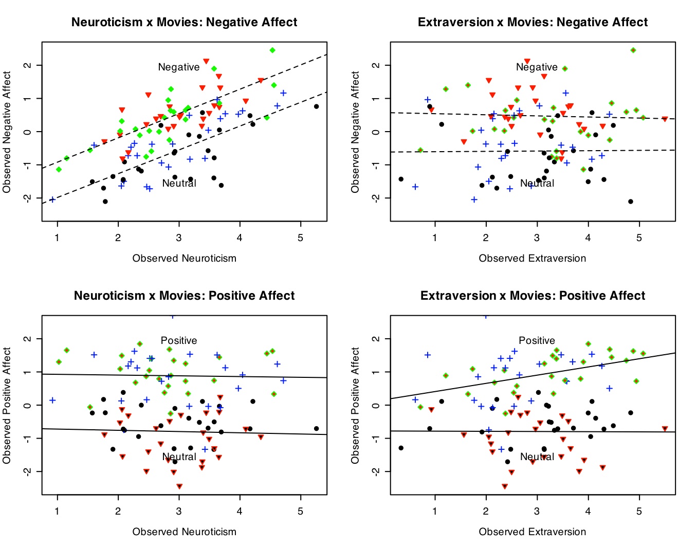
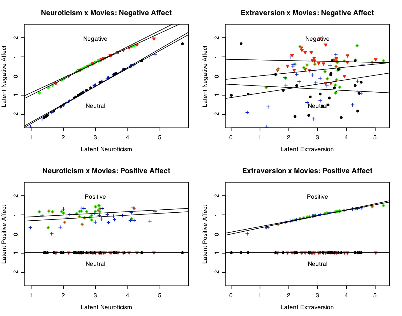
The best way to show this set of interactions is by a four panel graph. (Details on making this graph are given in the graphics section.) Note the clear additive effects of Neuroticism and Negative movies on Negative Affect (top left panel), the lack of an effect of Extraversion on Negative Affect (top right), the effect of positive movies on Positive affect (bottom panels), and the effect of extraversion by movie condition (bottom right). There is an interaction between movie type (reward x punishment) and affect measure, shown in the within subjects analysis.
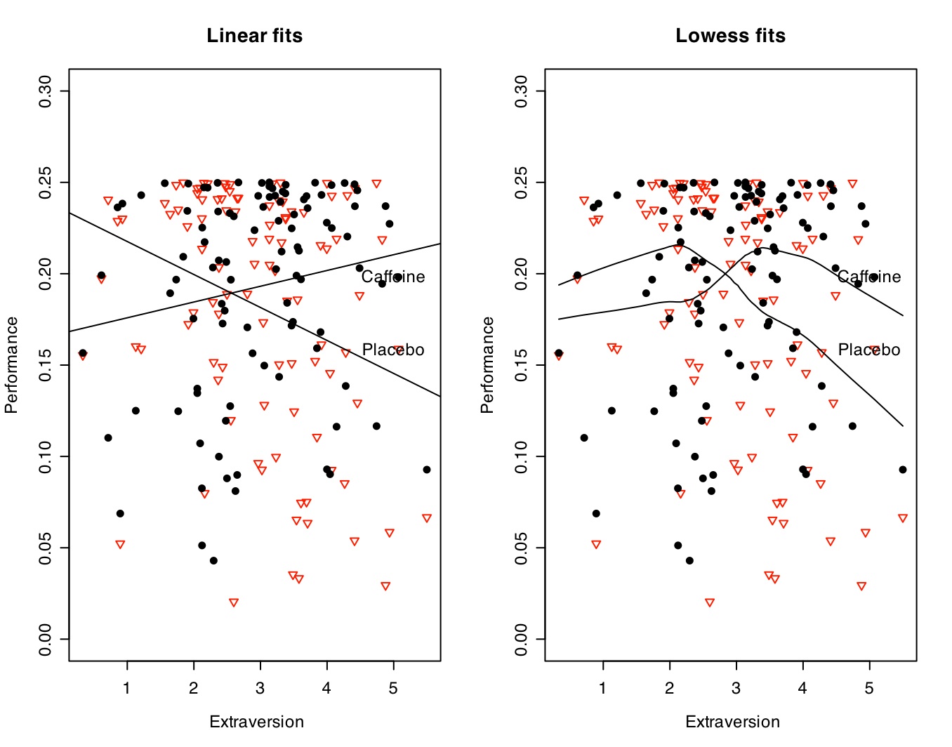
Study 4: The effect of caffeine and extraversion on cognitive performance
Analyse the drug by extraversion data. Since this is a within subjects design, we will need to rearrange the data slightly.
#repeated measures ANOVA
#this requires a bit more work, in that we need to string out the data

attach(drug.data)

drug.df <- data.frame(performance_plac,performance_caff)   #make this into a 2 column data frame
stacked.drug <- stack(drug.df)                 #string the data out for analysis
drug.design.df <- data.frame(stacked.drug,rbind(drug.data,drug.data),subj=gl(num,1,2*num))
#note that subject is a factor in the repeated measures design
#the gl() function creates the factors
#drug.design.df        #show the data frame to understand it
detach(drug.data)

mod10 <- aov(values ~ ind*extraversion+Error(subj),data=drug.design.df)
summary(mod10)


summary(mod10)

Error: subj
             Df  Sum Sq Mean Sq F value Pr(>F)
extraversion  1 0.00506 0.00506  1.4492 0.2316
Residuals    98 0.34197 0.00349

Error: Within
                 Df  Sum Sq Mean Sq F value   Pr(>F)
ind               1 0.00568 0.00568   1.506 0.222685
ind:extraversion  1 0.04068 0.04068  10.791 0.001415 **
Residuals        98 0.36940 0.00377
---
Signif. codes:  0 ‘***’ 0.001 ‘**’ 0.01 ‘*’ 0.05 ‘.’ 0.1 ‘ ’ 1
This can be shown graphically in two different ways. The left hand panel simply shows the two regression lines (Performance as a function of extraversion for Placebo and Caffeine conditions). This shows that performance declines with extraversion in the placebo condition and increases in the caffeine condition. This is the within subjects interaction with extraversion term in the regression analysis. The right hand panel clarifies this relationship by using a "lowess" smooth of the data, suggesting a curvilinear fit for both drug conditions with a difference of the peaks of the curves.
Graphical Data Summaries
Graphical presentations of the data make these results easier to understand. With not many subjects, it is useful to show the data points as well, but as the number of participants increases, it is probably better to show just the regression lines. Here we show the commands that made the graphs presented above.
For an overview of how to use R for graphics, consult the short guide to R, for detailed discussions of graphics in R, consult the many help pages for graphics.
#graphical output helps understand interactions
#the following code shows how to draw these graphs
#First, Figure 1


symb <- c(19,25,3,23)                              #choose some nice plotting symbols
colors <- c("black","red","green","blue")          #choose some nice colors

par(mfrow=c(1,2))     #specify the number of rows and columns in a multi panel graph


#make a two panel graph of the neuroticism x punishment study

attach(affect.data) 	#this gives us direct access to the variables
#first draw the latent results, fit them, and label them
plot(true_n,TrueNegAffect,pch=symb[punish],col=colors[punish],bg=colors[punish],cex=1.0,ylim =c(-2.5,2.5),ylab="Latent Negative Affect",
xlab="Latent Neuroticism",main="True relationships")               #show the data points
by(affect.data,punish,function(x) abline(lm(TrueNegAffect~true_n,data=x)))
text(3,-1.5,"Neutral")
text(3,2,"Negative")
by(affect.data,punish,function(x) summary(lm(PosAffect~extraversion,data=x),digits=2))

plot(neuroticism,NegAffect,pch=symb[punish],col=colors[punish],bg=colors[punish],cex=1.0,ylim =c(-2.5,2.5),ylab="Observed Negative Affect",
xlab="Observed Neuroticism", main="Observed relationships")               #show the data points
by(affect.data,punish,function(x) abline(lm(NegAffect~neuroticism,data=x)))
text(3,-2.3,"Neutral")
text(3,2,"Negative")
by(affect.data,punish,function(x) summary(lm(NegAffect~neuroticism,data=x),digits=2))
detach(affect.data)                 #otherwise, we have copies floating around


 Figure 1: The effect of negative feedback or a sad movie upon Negative Affect


#now do a 2 panel graph of the extraversion x reward study
#first draw the latent results, then the "real results"

attach(affect.data) 	#this gives us direct access to the variables
colors <- c("black","blue","green","red")
plot(true_e,TruePosAffect,pch=symb[reward],col=colors[reward],bg=colors[reward],cex=1.0,ylim =c(-2.5,2.5),ylab="Latent Positive Affect",
xlab="Latent extraversion",main="True relationships")               #show  the data points
by(affect.data,reward,function(x) abline(lm(TruePosAffect~true_e,data=x)))
text(3,-1.5,"Neutral")
text(3,2,"Positive")
by(affect.data,reward,function(x) summary(lm(PosAffect~extraversion,data=x),digits=2))

plot(extraversion,PosAffect,pch=symb[reward],col=colors[reward],bg=colors[reward],cex=1.0,ylim =c(-2.5,2.5),ylab="Observed Positive Affect",
xlab="Observed Extraversion", main="Observed relationships")               #show  the data points
by(affect.data,reward,function(x) abline(lm(PosAffect~extraversion,data=x)))
text(3,-2.3,"Neutral")
text(3,2,"Positive")
by(affect.data,reward,function(x) summary(lm(PosAffect~extraversion,data=x),digits=2))
detach(affect.data)                 #otherwise, we have copies floating around
Figure 2: The effect of positive feedback or a happy movie upon Positive Affect
Now, draw a 2 x 2 panel graph of the complete relationships. First we will do this for the latent (pure) data, and then for the observed data.
#graphical output helps understand interactions

attach(affect.data) 	#this gives us direct access to the variables

symb <- c(19,25,3,23)                              #choose some nice plotting symbols
colors <- c("black","red","blue","green")          #choose some nice colors

par(mfrow=c(2,2))
#make a four panel graph of the personality x film data
#the rows will be affect
#the columns personality variable
#The four separate lines in each graph represent the four movie conditions
#solid lines compare neutral vs. negative (threat) movies
#dashed lines compare neutral vs. positive (reward) movies

moviecond <- as.numeric(punish) + 2* as.numeric(reward) -2   #movie conditions
#movie conditions 1 = neutral   2 = punish alone  3= reward alone   4 = punish+reward

#first draw the latent results, fit them, and label them
plot(true_n,TrueNegAffect,pch=symb[moviecond],col=colors[moviecond],bg=colors[moviecond],cex=1.0,ylim =c(-2.5,2.5),ylab="Latent Negative Affect",
xlab="Latent Neuroticism",main="Neuroticism x Movies: Negative Affect")               #show  the data points

by(affect.data,moviecond,function(x) abline(lm(TrueNegAffect~true_n,data=x)))

text(3,-1.5,"Neutral")
text(3,2,"Negative")

plot(true_e,TrueNegAffect,pch=symb[moviecond],col=colors[moviecond],bg=colors[punish],cex=1.0,ylim =c(-2.5,2.5),ylab="Latent Negative Affect",
xlab="Latent Extraversion",main="Extraversion x Movies: Negative Affect")               #show  the data points
by(affect.data,moviecond,function(x) abline(lm(TrueNegAffect~true_e,data=x)))

text(3,-1.5,"Neutral")
text(3,2,"Negative")

plot(true_n,TruePosAffect,pch=symb[moviecond],col=colors[moviecond],bg=colors[reward],cex=1.0,ylim =c(-2.5,2.5),ylab="Latent Positive Affect",
xlab="Latent Neuroticism",main="Neuroticism x Movies: Positive Affect")               #show  the data points
by(affect.data,moviecond,function(x) abline(lm(TruePosAffect~true_n,data=x)))

text(3,-1.5,"Neutral")
text(3,2,"Positive")

plot(true_e,TruePosAffect,pch=symb[moviecond],col=colors[moviecond],bg=colors[reward],cex=1.0,ylim =c(-2.5,2.5),ylab="Latent Positive Affect",
xlab="Latent Extraversion",main="Extraversion x Movies: Positive Affect")               #show  the data points
by(affect.data,moviecond,function(x) abline(lm(TruePosAffect~true_e,data=x)))

text(3,-1.5,"Neutral")
text(3,2,"Positive")
The latent data (without error) show the effects of movie conditions upon positive and negative affect.
#now do it for the real data

symb <- c(19,25,3,23)                              #choose some nice plotting symbols
colors <- c("black","red","blue","green")          #choose some nice colors
attach(affect.data)

par(mfrow=c(2,2))
#make a four panel graph of the personality x film data
#the rows will be affect
#the columns personality variable
#The four separate lines in each graph represent the four movie conditions
#solid lines compare neutral vs. negative (threat) movies
#dashed lines compare neutral vs. positive (reward) movies

moviecond <- as.numeric(punish) + 2* as.numeric(reward) -2   #movie conditions
#movie conditions 1 = neutral   2 = punish alone  3= reward alone   4 = punish+reward

#first draw the latent results, fit them, and label them
plot(neuroticism,NegAffect,pch=symb[moviecond],col=colors[moviecond],bg=colors[moviecond],cex=1.0,ylim =c(-2.5,2.5),ylab="Observed Negative Affect",
xlab="Observed Neuroticism",main="Neuroticism x Movies: Negative Affect")               #show  the data points

by(affect.data,punish,function(x)      abline(lm(NegAffect~neuroticism,data=x),lty="dashed"))  #add regression slopes

text(3,-1.5,"Neutral")
text(3,2,"Negative")

plot(extraversion,NegAffect,pch=symb[moviecond],col=colors[moviecond],bg=colors[punish],cex=1.0,ylim =c(-2.5,2.5),ylab="Observed Negative Affect",
xlab="Observed Extraversion",main="Extraversion x Movies: Negative Affect")               #show  the data points
by(affect.data,punish,function(x) abline(lm(NegAffect~extraversion,data=x),lty="dashed"))

text(3,-1.5,"Neutral")
text(3,2,"Negative")


plot(neuroticism,PosAffect,pch=symb[moviecond],col=colors[moviecond],bg=colors[reward],cex=1.0,ylim =c(-2.5,2.5),ylab="Observed Positive Affect",
xlab="Observed Neuroticism",main="Neuroticism x Movies: Positive Affect")               #show  the data points
by(affect.data,reward,function(x) abline(lm(PosAffect~neuroticism,data=x)))

text(3,-1.5,"Neutral")
text(3,2,"Positive")

plot(extraversion,PosAffect,pch=symb[moviecond],col=colors[moviecond],bg=colors[reward],cex=1.0,ylim =c(-2.5,2.5),ylab="Observed Positive Affect",
xlab="Observed Extraversion",main="Extraversion x Movies: Positive Affect")               #show  the data points
by(affect.data,reward,function(x) abline(lm(PosAffect~extraversion,data=x)))

text(3,-1.5,"Neutral")
text(3,2,"Positive")

detach(affect.data)                 #otherwise, we have copies floating around


by(affect.data,punish,function(x) summary(lm(PosAffect~extraversion,data=x),digits=2))

plot(neuroticism,NegAffect,pch=symb[punish],col=colors[punish],bg=colors[punish],cex=1.0,ylim =c(-2.5,2.5),ylab="Observed Negative Affect",
xlab="Observed Neuroticism", main="Observed relationships")               #show  the data points
by(affect.data,punish,function(x) abline(lm(NegAffect~neuroticism,data=x)))
text(3,-2.3,"Neutral")
text(3,2,"Negative")
by(affect.data,punish,function(x)
summary(lm(NegAffect~neuroticism,data=x),digits=2))
detach(affect.data)                 #otherwise, we have copies floating around


#now do a 2 panel graph of the extraversion x reward study
#first draw the latent results, then the "real results"

attach(affect.data) 	#this gives us direct access to the variables
colors <- c("black","blue","green","red")
plot(true_e,TruePosAffect,pch=symb[reward],col=colors[reward],bg=colors[reward],cex=1.0,ylim =c(-2.5,2.5),ylab="Latent Positive Affect",
xlab="Latent extraversion",main="True relationships")               #show  the data points
by(affect.data,reward,function(x) abline(lm(TruePosAffect~true_e,data=x)))
text(3,-1.5,"Neutral")
text(3,2,"Positive")
by(affect.data,reward,function(x) summary(lm(PosAffect~extraversion,data=x),digits=2))

plot(extraversion,PosAffect,pch=symb[reward],col=colors[reward],bg=colors[reward],cex=1.0,ylim =c(-2.5,2.5),ylab="Observed Positive Affect",
xlab="Observed Extraversion", main="Observed relationships")               #show  the data points
by(affect.data,reward,function(x) abline(lm(PosAffect~extraversion,data=x)))
text(3,-2.3,"Neutral")
text(3,2,"Positive")
by(affect.data,reward,function(x) summary(lm(PosAffect~extraversion,data=x),digits=2))
detach(affect.data)                 #otherwise, we have copies floating around
The "real" data are much noiser than the latent data but the same pattern of interactions is still shown.
Show the extraversion x caffeine graph. Note how we are fitting both linear and lowess fits to the data. Which provides a better description?
#graph the caffeine and placebo by extraversion data

attach(drug.design.df)


par(mfrow=c(1,2))                            #set the number of rows and columns
symb <- c(19,25,3,23)                              #choose some nice plotting symbols
colors <- c("black","red","blue","green")          #choose some nice colors

plot(extraversion,values,pch=symb[ind],col=colors[ind],cex=1.0,ylim =c(-0,.3),ylab="Performance",xlab=" Extraversion",main="Linear fits")
by(drug.design.df,ind,function(x) abline(lm(values~extraversion,data=x)))
text(5,.16,"Placebo")
text(5,.20,"Caffeine")

plot(extraversion,values,pch=symb[ind],col=colors[ind],cex=1.0,ylim =c(-0,.3),ylab="Performance",xlab=" Extraversion",main="Lowess fits")

text(5,.16,"Placebo")
text(5,.2,"Caffeine")
lines(lowess(performance_plac~extraversion))
lines(lowess(performance_caff~extraversion))

detach(drug.design.df)   #otherwise we have copies floating around
Multiple Dependent Measures- Multilevel or Mixed Model approaches
Traditionally, when examining several dependent variables (e.g., positive and negative affect), one might be interested in whether there is a difference in the effects depending upon which dependent variable is examined. That is, is there an interaction of dependent variable by some treatment? Although traditionally repeated measures ANOVA has been used (see above), more recent treatments are using a variety of procedures that generically are studying "mixed effects". Known as HLM, Proc Mixed, or just nmle, these procedures attempt to model the data at multiple levels, the subject level (where the repeated measures occur) and at a higher level (other characteristics of the subject.) See Pinheiro, J. C. & Bates, D.M. (2000) Mixed-effects models in S and S-Plus. Springer, New York. for more detail.
##Newer developments allow for mixed model estimates

library(nmle)       #we need to use the nmle package

mod.lme <- lme(values ~ind*reward*punish, random = ~1 |subj,data=design.df)
mod.lme <- lme(values ~ind*reward*punish, random = ~1 |neuroticism/subj,data=design.df)
mod.lme <- lme(values ~ind*reward*punish*extraversion*neuroticism , random = ~1 |subj,data=design.df)
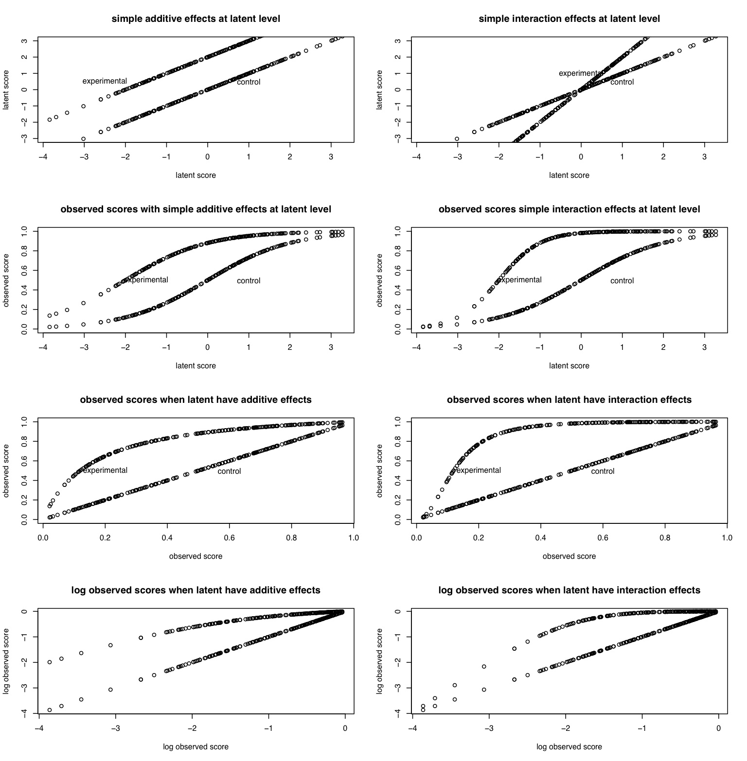
Simulation 3: Challenges in measurement
A serious problem in inference about main effects and interactions is the relationship between observed variables and latent variables. If the OV is a monotonic but non linear function of the latent variable, and the latent variable is a function of some latent trait as well as some experimental manipulation, then it is likely that some observed interactions are due to the non linearity of the function rather than a true interaction.
In the chapter we discuss the problem of inference and scaling artifact. The R code for drawing the graph presented there is shown here.

#use curve to draw theoretical curves
#use margin control to make multi-panel graphs
#note that we scale the entire figure from 0 to 100


#pdf("revelle.figure3.pdf",height=6,width=9)

par(mfrow=c(1,3))
par(mar=c(5,2,4,0))
curve(100/(1+exp(-x+2)),0,1,ylim=c(0,100),xaxp=c(0,1,1),xlab="Time during Year",main="Reading", cex=1.5)
curve(100/(1+exp(-x+3)),0,1,add=TRUE)
curve(100/(1+exp(-x+1)),0,1,add=TRUE)
text(.5,5,"Junior College")
text(.5,15,"Non selective")
text(.5,35,"Selective")


par(mar=c(5,0,4,0))
curve(100/(1+exp(-x-2)),-0,1,ylim=c(0,100),yaxt="n",xaxp=c(0,1,1),xlab="Time during Year",main="Mathematics")
curve(100/(1+exp(-x-3)),-0,1,add=TRUE)
curve(100/(1+exp(-x-1)),-0,1,add=TRUE)
text(.5,75,"Junior College")
text(.5,90,"Non selective")
text(.5,100,"Selective")


par(mar=c(5,0,4,1))
curve(100/(1+exp(-x-2)),-3,3,ylim=c(0,100),xlim = c(-2.5,2.5),yaxt="n",xlab="latent growth",main="Observed by Latent",lty="dotted")
#curve(100/(1+exp(-x-3)),-3,3,add=TRUE,lty="dashed")
#curve(100/(1+exp(-x+3)),-3,3,add=TRUE,lty="dashed")
curve(100/(1+exp(-x+2)),-3,3,add=TRUE,lty="dotted")
#curve(100/(1+exp(-x-1)),-3,3,add=TRUE,lty="dashed")
#curve(100/(1+exp(-x+1)),-3,3,add=TRUE,lty="dashed")
curve(100/(1+exp(-x-2)),1,2,add=TRUE,lwd=4)
curve(100/(1+exp(-x+2)),1,2,add=TRUE,lwd=4)
curve(100/(1+exp(-x+2)),-0,1,add=TRUE)
curve(100/(1+exp(-x-2)),-0,1,add=TRUE)
curve(100/(1+exp(-x+2)),-1,0,add=TRUE,lty="dashed",lwd=2)
curve(100/(1+exp(-x-2)),-1,0,add=TRUE,lty="dashed",lwd=2)

text(.2,5,"Junior College")
text(1,15,"Non selective")
text(2,35,"Selective")
text(.2,80,"Junior College")
text(1,90,"Non selective")
text(1.8,95,"Selective")
#dev.off()
In the following simulations this point is made somewhat clearer. Following the work in Item Response Theory, the OV is a logistic function of a latent trait. Situational manipulations are simulated by shifts along the latent trait. Latent interactions are created as product terms.
#measurement issues are a serious problem in inference
#The following code generates raw data for latent true scores
#and the creates observed scores as logistic transforms of latent scores
#Both additive and interactive effects are shown

#first some arbitrary constants
nsubjects <- 200
additive <- -2
interaction <- 2
error <- 1
constant <- 0   #additive constant to make all variable positive

theta <- rnorm(nsubjects) + error*rnorm(nsubjects) + constant   #basic trait has error

addtheta <- theta - additive
interact <- theta*interaction
observed1 <- 1/(1+exp(-theta + constant))
observed2 <- 1/(1+exp(additive - theta + constant))
observed3 <- 1/(1+exp(interaction*(additive -theta + constant)))
mydata <- data.frame(theta,addtheta,interact,observed1,observed2,observed3)
mydata.log <- log(mydata)
describe(mydata)
pairs.panels(mydata)


op <- par(mfrow=c(4,2))
plot(theta,theta,xlab="latent score", ylab="latent score",main="simple additive effects at latent level",ylim=c(-3,3))
points(theta,addtheta)
text(1,.5,"control")
text(-2.5,.5,"experimental")

plot(theta,theta ,xlab="latent score", ylab="latent score",main="simple interaction effects at latent level",ylim=c(-3,3))
points(theta,interact)
text(1,.5,"control")
text(0,1,"experimental")

plot(theta,observed1,xlab="latent score", ylab="observed score",main="observed scores with simple additive effects at latent level",ylim=c(0,1))
points(theta,observed2)
text(1,.5,"control")
text(-1.5,.5,"experimental")

plot(theta,observed1,xlab="latent score", ylab="observed score",main="observed scores simple interaction effects at latent level",ylim=c(0,1))
points(theta,observed3)
text(1,.5,"control")
text(-1.5,.5,"experimental")

plot(observed1,observed1,xlab="observed score", ylab="observed score",main="observed scores when latent have additive effects",ylim=c(0,1))
points(observed1,observed2)
text(.6,.5,"control")
text(.2,.5,"experimental")

plot(observed1,observed1,xlab="observed score", ylab="observed score",main="observed scores when latent have interaction effects",ylim=c(0,1))
points(observed1,observed3)
text(.6,.5,"control")
text(.2,.5,"experimental")


plot(log(observed1),log(observed1),xlab="log observed score", ylab="log observed score",main="log observed scores when latent have additive effects")
points(log(observed1),log(observed2))
text(.6,.5,"control")
text(.2,.5,"experimental")

plot(log(observed1),log(observed1),xlab="log observed score", ylab="log observed score",main="log observed scores when latent have interaction effects")
points(log(observed1),log(observed3))
text(.6,.5,"control")
text(.2,.5,"experimental")
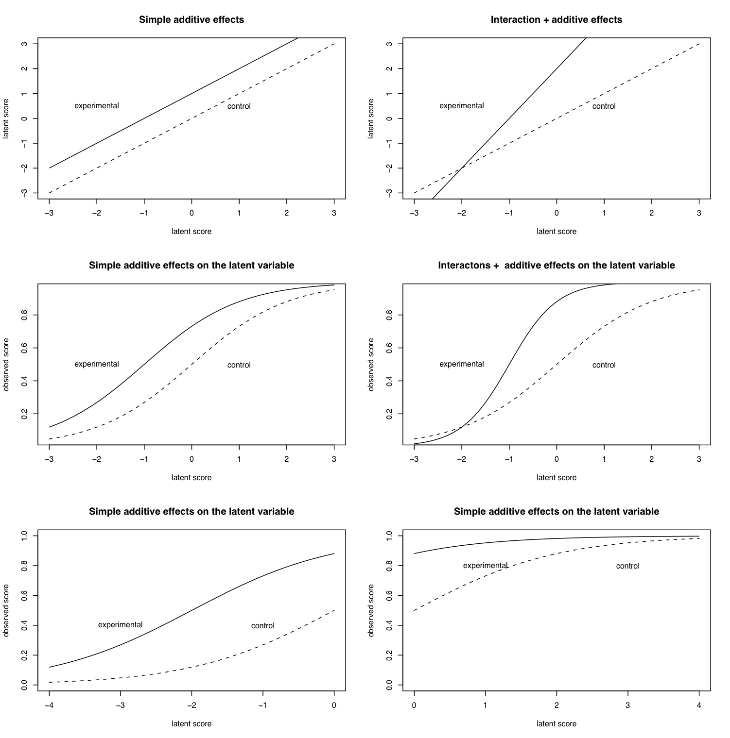
logistic <- function(x,a=0,b=1) {1/(1+exp(b*(a-x)))}
raw <- function(x) {x}

op <- par(mfrow=c(3,2))

curve(raw(x),-3,3,101,ylab ="latent score",xlab="latent score",lty="dashed")
curve(raw(x+1),-3,3,101,add=T)
#curve(raw(x-1),-3,3,101,add=T)
text(1,.5,"control")
text(-2,.5,"experimental")
title("Simple additive effects")

curve(raw(x),-3,3,101,ylab ="latent score",xlab="latent score",lty="dashed")
#curve(raw(x*2),-3,3,101,add=T)
curve(raw((x+1)*2),-3,3,101,add=T)
text(1,.5,"control")
text(-2,.5,"experimental")
title("Interaction + additive effects")


curve(logistic(x),-3,3,101,xlab="latent score", ylab="observed score",lty="dashed")
curve(logistic(x,a=-1),-3,3,101,add=T)
#curve(logistic(x,a=-1),-3,3,101,add=T)
text(1,.5,"control")
text(-2,.5,"experimental")
title("Simple additive effects on the latent variable")

curve(logistic(x), -3,3,101,xlab="latent score", ylab="observed score",lty="dashed")
#curve(logistic(x,b=2), -3,3,101,add=T)
curve(logistic(x,a=-1,b=2),-3,3,101,add=T)
text(1,.5,"control")
text(-2,.5,"experimental")
title("Interactons +  additive effects on the latent variable")

curve(logistic(x),-4,0,101,xlab="latent score", ylab="observed score",lty="dashed",ylim=c(0,1))
curve(logistic(x,a=-2),-4,0,101,add=T)
#curve(logistic(x,a=-1),-4,0,101,add=T)
text(-1,.4,"control")
text(-3,.4,"experimental")
title("Simple additive effects on the latent variable")

curve(logistic(x),0,4,101,xlab="latent score", ylab="observed score",lty="dashed",ylim=c(0,1))
curve(logistic(x,a=-2),0,4,101,add=T)
#curve(logistic(x,a=-1),0,4,101,add=T)
text(3,.8,"control")
text(1,.8,"experimental")
title("Simple additive effects on the latent variable")
mtext("The effect of scaling on inference",3,outer=TRUE,line=1,cex=1.5)
The reader is encouraged to take the code in these simulations and to generate more cases, with different parameters to see what happens.
part of a guide to R
Version of July 10, 2006
William Revelle
Department of Psychology
Northwestern University