Using R for personality research
This is a very brief guide to help students in a personality research course make use of the R statistical language to analyze some of the data they have collected. For more extensive tutorials of R in psychology, see my somewhat longer tutorial as well as the excellent tutorial by Jonathan Baron and Yuelin Li.
(Note that the blue text may be directly copied into R)
12 simple steps
- Install R on your computer or go to a machine that has it
- Install the psych and psychTools packages using the package installer. Note, that you only need to do this once.
- Activate psych by using the library(psych) command
- Enter your data using a text editor and save as a text file (perhaps comma delimited if using Excel)
- Read the data file (read.file) or copy and paste from the clipboard (read.clipboard).
- Find basic descriptive statistics (e.g., means, standard deviations, minimum and maxima) using describe.
- Prepare a simple descriptive graph (e.g, violin plot or box.plot) of your variables
- Find the correlation matrix to give an overview of relationships using lowerCor or corPlot or pairs.panels.
- If you have an experimental variable, do the appropriate multiple regression lm or lmCor.
- If you want to do a factor analysis or principal components analysis, use the fa or principal functions.
- To score items and create scale(s) and find various reliability estimates, use scoreItems and perhaps omega.
- Graph the results
Getting started
Installing R on your computer
Many labs have R already installed. However, to do analyses on your own machine, you will need to download the R program from the R project and install it yourself. Go to the R home page and then choose the Download from CRAN (Comprehensive R Archive Network) option. This will take you to list of mirror sites around the world. A convenient mirror for those of us at Northwestern is at UCLA: http://cran.stat.ucla.edu/ You may download the Windows, Linux, or Mac versions at this site. Installation differs across platforms but, at least for a Mac, is very easy.
Run R with a text editor to save your commands for later use.
R is case sensitive and does not give overly useful diagnostic messages. If you get an error message, don't be flustered but rather be patient and try the command again using the correct spelling for the command.
Help and Guidance
When in doubt, use the help () function. This is identical to the ? function where function is what you want to know about. e.g.,
? read.table    #ask for help in using the read.table function  -- see the answer in its own window
#or
help (read.table) #another way of asking for help.  - see the window
Useful additions to R
One of the advantages of R is that it can be supplemented with additional programs that are included as "packages" using the package manager. (e.g., sem does structural equation modeling) or that can be added using the "source" command. Some additions to the basic program that are particularly useful for personality research can be added by
source("http://personality-project.org/r/useful.r")
Even better is installing the psych package. This includes most of the functions that I have found most useful for personality research. They have been organized into the psych package. Using the package installer option, go to the CRAN site and download and install psych.
install.packages("psych")
This needs to be done just once. However, if you want to use the functions in the psych package, you will need to make it active every time you start R. For an introduction to the psych package, read the vignette
library("psych")
Entering or getting the data
For most data analysis, rather than manually enter the data into R, it is probably more convenient to use a spreadsheet (e.g., Excel or OpenOffice) as a data editor, save as a tab or comma delimited file, and then read the data. Most of the examples in this tutorial assume that the data have been entered this way. Many of the examples in the help menus have small data sets entered using the c() command or created on the fly.
For the example, we read data from a remote file server for several hundred subjects on 13 personality scales (5 from the Eysenck Personality Inventory (EPI), 5 from a Big Five Inventory (BFI) ,1 Beck Depression, and two anxiety scales). The file is structured normally, i.e. rows represent different subjects, columns different variables, and the first row gives subject labels. Had we saved this file as comma delimited, we would add the separation (sep=",") parameter.
To read a file from your local machine, change the datafilename to specify the path to the data. A simple trick on the Mac is to store the datafile on your desktop. Thus the path is "Desktop/myfilename".
#specify the name and address of the remote file
datafilename="http://personality-project.org/r/datasets/maps.mixx.epi.bfi.data"

#If I want to read a datafile from my desktop
datafilename="Desktop/epi.big5.txt"

#now read the data file
person.data =read.table(datafilename,header=TRUE)  #read the data file

#Alternatively, to read in a comma delimited file:
#data =read.table(datafilename,header=TRUE,sep=",")


names(person.data)  #list the names of the variables
attach(person.data)  #makes the variables available for later analysis


#results in this output

datafilename="Desktop/epi.big5.txt"
>
> #now read the data file
> person.data =read.table(datafilename,header=TRUE)  #read the data file
> names(person.data)  #list the names of the variables
 [1] "epiE"     "epiS"     "epiImp"   "epilie"   "epiNeur"  "bfagree"  "bfcon"    "bfext"    "bfneur"   "bfopen"   "bdi"      "traitanx"
[13] "stateanx"
> attach(person.data)  #makes the variables available for later analysis
The data are now in the data.table "person.data". Tables allow one to have columns that are either numeric or alphanumeric. To list single subjects, to choose subjects meeting certain criteria, or to recode data, see the longer tutorial.
Descriptive Statistics
Basic descriptive statistics are most easily reported by using the summary, means and Standard Deviations (sd) commands. Using the describe function available in the psych package produces more useful results. Graphical displays that also capture this are available as a boxplot.
summary(person.data)  #print out the min, max, range, mean, median, etc. of the data

round(mean(person.data),2)   #means of all variables, rounded to 2 decimals
round(sd(person.data),2)      #standard deviations, rounded to 2 decimals

results in this output

summary(person.data)  #print out the min, max, range, mean, median, etc. of the data
      epiE            epiS            epiImp          epilie         epiNeur         bfagree          bfcon           bfext
 Min.   : 1.00   Min.   : 0.000   Min.   :0.000   Min.   :0.000   Min.   : 0.00   Min.   : 74.0   Min.   : 53.0   Min.   :  8.0
 1st Qu.:11.00   1st Qu.: 6.000   1st Qu.:3.000   1st Qu.:1.000   1st Qu.: 7.00   1st Qu.:112.0   1st Qu.: 99.0   1st Qu.: 87.5
 Median :14.00   Median : 8.000   Median :4.000   Median :2.000   Median :10.00   Median :126.0   Median :114.0   Median :104.0
 Mean   :13.33   Mean   : 7.584   Mean   :4.368   Mean   :2.377   Mean   :10.41   Mean   :125.0   Mean   :113.3   Mean   :102.2
 3rd Qu.:16.00   3rd Qu.: 9.500   3rd Qu.:6.000   3rd Qu.:3.000   3rd Qu.:14.00   3rd Qu.:136.5   3rd Qu.:128.5   3rd Qu.:118.0
 Max.   :22.00   Max.   :13.000   Max.   :9.000   Max.   :7.000   Max.   :23.00   Max.   :167.0   Max.   :178.0   Max.   :168.0
     bfneur           bfopen           bdi            traitanx        stateanx
 Min.   : 34.00   Min.   : 73.0   Min.   : 0.000   Min.   :22.00   Min.   :21.00
 1st Qu.: 70.00   1st Qu.:110.0   1st Qu.: 3.000   1st Qu.:32.00   1st Qu.:32.00
 Median : 90.00   Median :125.0   Median : 6.000   Median :38.00   Median :38.00
 Mean   : 87.97   Mean   :123.4   Mean   : 6.779   Mean   :39.01   Mean   :39.85
 3rd Qu.:104.00   3rd Qu.:136.5   3rd Qu.: 9.000   3rd Qu.:44.00   3rd Qu.:46.50
 Max.   :152.00   Max.   :173.0   Max.   :27.000   Max.   :71.00   Max.   :79.00
>
> round(mean(person.data),2)   #means of all variables, rounded to 2 decimals
    epiE     epiS   epiImp   epilie  epiNeur  bfagree    bfcon    bfext   bfneur   bfopen      bdi traitanx stateanx
   13.33     7.58     4.37     2.38    10.41   125.00   113.25   102.18    87.97   123.43     6.78    39.01    39.85
> round(sd(person.data),2)      #standard deviations, rounded to 2 decimals
    epiE     epiS   epiImp   epilie  epiNeur  bfagree    bfcon    bfext   bfneur   bfopen      bdi traitanx stateanx
    4.14     2.69     1.88     1.50     4.90    18.14    21.88    26.45    23.34    20.51     5.78     9.52    11.48
>
Using the describe function (found in the psych package) provides somewhat more readable output that is convenient for reporting in tables:
 describe(person.data)


         var   n   mean    sd median   mad min max range  skew kurtosis   se
epiE       1 231  13.33  4.14     14  4.45   1  22    21 -0.33    -0.06 0.27
epiS       2 231   7.58  2.69      8  2.97   0  13    13 -0.57    -0.02 0.18
epiImp     3 231   4.37  1.88      4  1.48   0   9     9  0.06    -0.62 0.12
epilie     4 231   2.38  1.50      2  1.48   0   7     7  0.66     0.24 0.10
epiNeur    5 231  10.41  4.90     10  4.45   0  23    23  0.06    -0.50 0.32
bfagree    6 231 125.00 18.14    126 17.79  74 167    93 -0.21    -0.27 1.19
bfcon      7 231 113.25 21.88    114 22.24  53 178   125 -0.02     0.23 1.44
bfext      8 231 102.18 26.45    104 22.24   8 168   160 -0.41     0.51 1.74
bfneur     9 231  87.97 23.34     90 23.72  34 152   118  0.07    -0.55 1.54
bfopen    10 231 123.43 20.51    125 20.76  73 173   100 -0.16    -0.16 1.35
bdi       11 231   6.78  5.78      6  4.45   0  27    27  1.29     1.50 0.38
traitanx  12 231  39.01  9.52     38  8.90  22  71    49  0.67     0.47 0.63
stateanx  13 231  39.85 11.48     38 10.38  21  79    58  0.72    -0.01 0.76
The describe.by function combines describe with with the by function to provide evem more detailed tables. This example reports descriptive statistics for subjects with lie scores < 3 and those >= 3. The second element in the by command could be a categorical variable (e.g., sex).
describeBy(person.data,person.data$epilie <3)

describeBy(person.data,person.data$epilie <3)
group: FALSE
         var  n   mean    sd median   mad min max range  skew kurtosis   se
epiE       1 90  12.64  4.00   13.0  2.97   1  21    20 -0.68     0.49 0.42
epiS       2 90   7.61  2.81    8.0  2.97   0  13    13 -0.57    -0.04 0.30
epiImp     3 90   3.97  1.67    4.0  1.48   1   8     7  0.15    -0.51 0.18
epilie     4 90   3.89  1.08    4.0  1.48   3   7     4  1.02     0.12 0.11
epiNeur    5 90   9.33  5.20    9.0  5.93   0  20    20  0.03    -0.95 0.55
bfagree    6 90 128.12 16.55  129.0 13.34  87 167    80 -0.08    -0.22 1.74
bfcon      7 90 117.56 20.46  118.0 19.27  58 178   120 -0.01     0.52 2.16
bfext      8 90 100.88 25.24  101.0 21.50  24 151   127 -0.24     0.30 2.66
bfneur     9 90  82.22 22.80   81.5 27.43  35 144   109  0.27    -0.65 2.40
bfopen    10 90 121.97 20.55  121.0 17.79  75 172    97 -0.14    -0.42 2.17
bdi       11 90   5.77  4.71    5.0  4.45   0  24    24  1.27     2.47 0.50
traitanx  12 90  37.01  9.06   36.0 10.38  22  71    49  0.70     0.92 0.95
stateanx  13 90  38.41 11.36   36.5 12.60  21  69    48  0.59    -0.42 1.20
--------------------------------------------------------------------------------------------------------------------------------
group: TRUE
         var   n   mean    sd median   mad min max range  skew kurtosis   se
epiE       1 141  13.77  4.17     14  4.45   4  22    18 -0.17    -0.59 0.35
epiS       2 141   7.57  2.62      8  2.97   1  13    12 -0.56    -0.06 0.22
epiImp     3 141   4.62  1.97      5  2.97   0   9     9 -0.08    -0.70 0.17
epilie     4 141   1.41  0.73      2  0.00   0   2     2 -0.80    -0.73 0.06
epiNeur    5 141  11.10  4.59     10  4.45   0  23    23  0.22    -0.33 0.39
bfagree    6 141 123.00 18.88    124 20.76  74 165    91 -0.19    -0.43 1.59
bfcon      7 141 110.50 22.38    111 22.24  53 176   123  0.03     0.08 1.88
bfext      8 141 103.01 27.25    105 23.72   8 168   160 -0.51     0.58 2.29
bfneur     9 141  91.64 23.01     94 23.72  34 152   118 -0.05    -0.38 1.94
bfopen    10 141 124.36 20.50    126 19.27  73 173   100 -0.17    -0.03 1.73
bdi       11 141   7.43  6.29      6  5.93   0  27    27  1.16     0.76 0.53
traitanx  12 141  40.28  9.62     39  8.90  23  71    48  0.65     0.19 0.81
stateanx  13 141  40.77 11.51     39 10.38  23  79    56  0.80     0.12 0.97
Simple Graphs
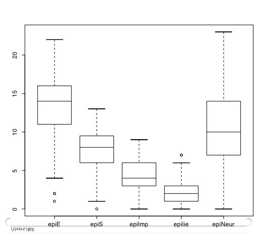
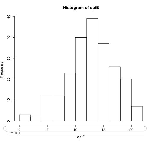
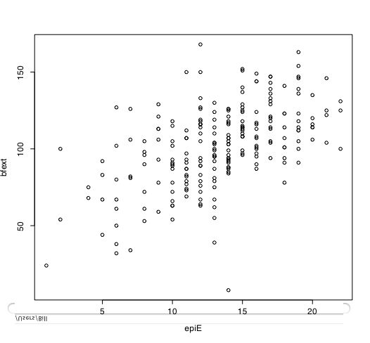
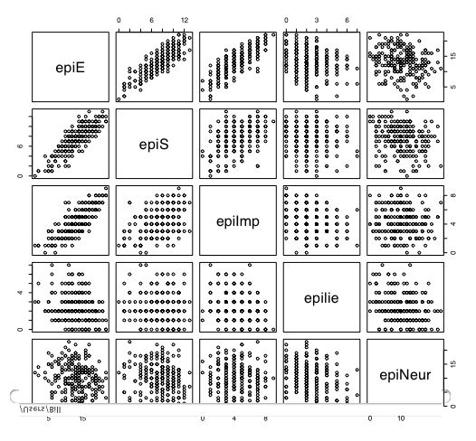
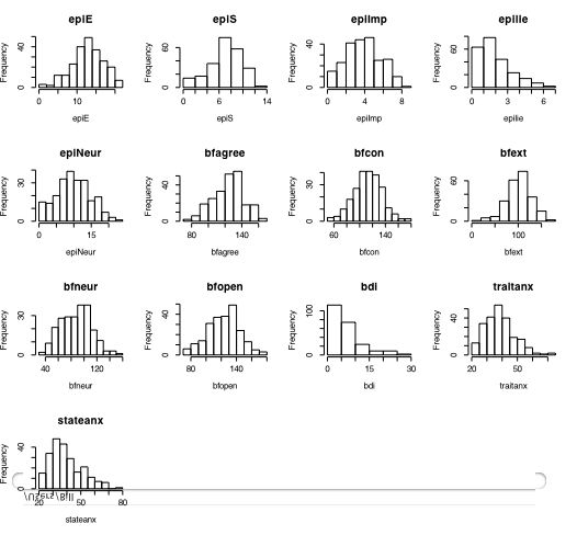
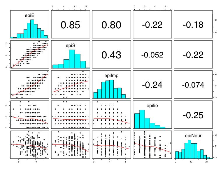
Another way of describing the data is to graph it. boxplot show the top and bottom quartiles, medians, and the "hinges". histograms show the distribution in more detail. The pairs command draws a matrix of scatter plots. (Note that I do this just for 5 variables to make it more readable).
boxplot(person.data[1:5]) #show a boxplot of the first 5 variables
hist(epiE)   #draws a histogram of the extraversion scores
plot(epiE,bfext) #show the scatter plot of two ways of measuring extraversion
pairs(person.data[1:5])   #draw a matrix of scatter plots for the first 5 variables
multi.hist(person.data) #draw the histograms for all variables
pairs.panels(person.data[1:5]) #draws scatterplots, histograms, and shows correlations  (source found in the psych package)
Resulting in the following figures:
One can create small functions to execute a number of commands at once. These functions can then be used for different sets of inputs. Examples of this may be found in the useful.r page.
Graphical output goes to a graphics window. This may be saved as a pdf using the save command (in the menus) and then printed in another document. On a mac, a new graphics window may be created by the quartz(height=9, width=6) command (height and width specified for nice looking output on a printer.)
quartz(height=9, width=6)
Correlations
The relationship between variables is seen graphically in the pairs command (see above). It is quantified with the Pearson Correlation. In case of missing values, it is necesary to specify that you want to use complete cases or pairwise deleted cases. Without rounding, the output is to 5 decimals. Rounding to 2 decimals is most appropriate.
round(cor(person.data,use="pairwise"),2)  #find the correlation matrix rounded to 2 decimals


Which produces this output:

          epiE  epiS epiImp epilie epiNeur bfagree bfcon bfext bfneur bfopen   bdi traitanx stateanx
epiE      1.00  0.85   0.80  -0.22   -0.18    0.18 -0.11  0.54  -0.09   0.14 -0.16    -0.23    -0.13
epiS      0.85  1.00   0.43  -0.05   -0.22    0.20  0.05  0.58  -0.07   0.15 -0.13    -0.26    -0.12
epiImp    0.80  0.43   1.00  -0.24   -0.07    0.08 -0.24  0.35  -0.09   0.07 -0.11    -0.12    -0.09
epilie   -0.22 -0.05  -0.24   1.00   -0.25    0.17  0.23 -0.04  -0.22  -0.03 -0.20    -0.23    -0.15
epiNeur  -0.18 -0.22  -0.07  -0.25    1.00   -0.08 -0.13 -0.17   0.63   0.09  0.58     0.73     0.49
bfagree   0.18  0.20   0.08   0.17   -0.08    1.00  0.45  0.48  -0.04   0.39 -0.14    -0.31    -0.19
bfcon    -0.11  0.05  -0.24   0.23   -0.13    0.45  1.00  0.27   0.04   0.31 -0.18    -0.29    -0.14
bfext     0.54  0.58   0.35  -0.04   -0.17    0.48  0.27  1.00   0.04   0.46 -0.14    -0.39    -0.15
bfneur   -0.09 -0.07  -0.09  -0.22    0.63   -0.04  0.04  0.04   1.00   0.29  0.47     0.59     0.49
bfopen    0.14  0.15   0.07  -0.03    0.09    0.39  0.31  0.46   0.29   1.00 -0.08    -0.11    -0.04
bdi      -0.16 -0.13  -0.11  -0.20    0.58   -0.14 -0.18 -0.14   0.47  -0.08  1.00     0.65     0.61
traitanx -0.23 -0.26  -0.12  -0.23    0.73   -0.31 -0.29 -0.39   0.59  -0.11  0.65     1.00     0.57
stateanx -0.13 -0.12  -0.09  -0.15    0.49   -0.19 -0.14 -0.15   0.49  -0.04  0.61     0.57     1.00
Alernatively, the lowerCor function in psych will automatically use pairwise complete, round to 2 decimals and abbreviate column names so they line up.
lowerCor(person.data)  #find the correlation matrix rounded to 2 decimals

         epiE  epiS  epImp epili epiNr bfagr bfcon bfext bfner bfopn bdi   trtnx sttnx
epiE      1.00
epiS      0.85  1.00
epiImp    0.80  0.43  1.00
epilie   -0.22 -0.05 -0.24  1.00
epiNeur  -0.18 -0.22 -0.07 -0.25  1.00
bfagree   0.18  0.20  0.08  0.17 -0.08  1.00
bfcon    -0.11  0.05 -0.24  0.23 -0.13  0.45  1.00
bfext     0.54  0.58  0.35 -0.04 -0.17  0.48  0.27  1.00
bfneur   -0.09 -0.07 -0.09 -0.22  0.63 -0.04  0.04  0.04  1.00
bfopen    0.14  0.15  0.07 -0.03  0.09  0.39  0.31  0.46  0.29  1.00
bdi      -0.16 -0.13 -0.11 -0.20  0.58 -0.14 -0.18 -0.14  0.47 -0.08  1.00
traitanx -0.23 -0.26 -0.12 -0.23  0.73 -0.31 -0.29 -0.39  0.59 -0.11  0.65  1.00
stateanx -0.13 -0.12 -0.09 -0.15  0.49 -0.19 -0.14 -0.15  0.49 -0.04  0.61  0.57  1.00
Regression
Correlations allow us to see the relationship between pairs of variables. Multiple correlation examines how well a set of predictor variables can predict a single dependent variable. The influence of each predictor variable is reported independently of the other predictor variables.
A simple case of multiple correlation is predicting depression as a function of Neuroticism and Anxiety. From the correlations found above, we know that both of these are related to depression. But about their joint effect? We use the linear model command (lm) to test for their joint linear effect.
model1=lm(bdi~epiNeur,data=person.data)
summary(model1)

model2=lm(bdi~epiNeur+traitanx,data=person.data)
summary(model2)


Which gives the conventional output:

model1=lm(bdi~epiNeur,data=person.data)
> summary(model1)

Call:
lm(formula = bdi ~ epiNeur, data = person.data)

Residuals:
     Min       1Q   Median       3Q      Max
-11.9548  -3.1577  -0.7707   2.0452  16.4092

Coefficients:
            Estimate Std. Error t value Pr(>|t|)
(Intercept) -0.32129    0.73070   -0.44     0.66
epiNeur      0.68200    0.06353   10.74   <2e-16 ***
---
Signif. codes:  0 `***' 0.001 `**' 0.01 `*' 0.05 `.' 0.1 ` ' 1

Residual standard error: 4.721 on 229 degrees of freedom
Multiple R-Squared: 0.3348,	Adjusted R-squared: 0.3319
F-statistic: 115.3 on 1 and 229 DF,  p-value: < 2.2e-16

>
> model2=lm(bdi~epiNeur+traitanx,data=person.data)
> summary(model2)

Call:
lm(formula = bdi ~ epiNeur + traitanx, data = person.data)

Residuals:
     Min       1Q   Median       3Q      Max
-12.0288  -2.6848  -0.5121   1.9823  13.3081

Coefficients:
            Estimate Std. Error t value Pr(>|t|)
(Intercept) -7.63779    1.24729  -6.124 3.97e-09 ***
epiNeur      0.25506    0.08448   3.019  0.00282 **
traitanx     0.30151    0.04347   6.935 4.13e-11 ***
---
Signif. codes:  0 `***' 0.001 `**' 0.01 `*' 0.05 `.' 0.1 ` ' 1

Residual standard error: 4.299 on 228 degrees of freedom
Multiple R-Squared: 0.4507,	Adjusted R-squared: 0.4459
F-statistic: 93.53 on 2 and 228 DF,  p-value: < 2.2e-16
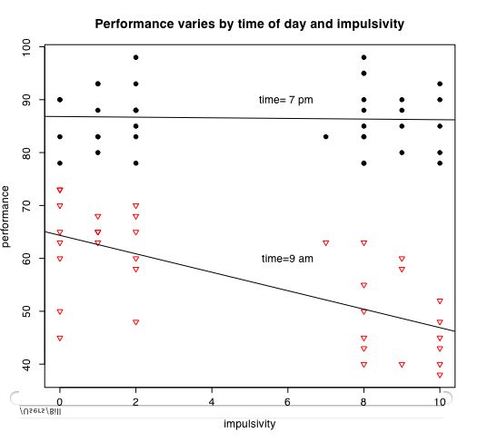
Graphing interactions
The next set of instructions allow us to consider the interaction of categorical variables with continuous variables. The data are from a simulation of performance varying by time of day and impulsivity.
#datafilename="Desktop/simulations.txt"    # my local copy of the data file
datafilename="http://personality-project.org/r/datasets/simulations.txt"  #web copy of data file
person.data =read.table(datafilename,header=TRUE)  #read the data file
attach(person.data)     #make the person.data the active set

#the next commands allow for a more generic set of plotting commands

DV=performance   #The Dependent Variable
IV1=impulsivity  #continuous Independent Variable
IV2=time        #categorical Independent Variable

mydata=data.frame(DV,IV1,IV2)   #put them together into one data frame
attach(mydata)

zmydata=data.frame(scale(mydata))             #convert the data to standard scores to do the regression analysis
                                              #this makes the interaction term independent of the main effects
model=lm(DV~IV1+IV2+ IV1*IV2,data=zmydata)    #test the main effects of IV1 and IV2 and the interaction of IV1 and IV2
print(model)              #just show the coefficients
summary(model)            #show the coefficients as well as the probability estimates for the coefficients


by(mydata,IV2,function(x) summary(lm(DV~IV1,data=x))) #give the summary stats for the regression DV~IV1 for each value of IV2

par(mfrow=c(1,1))                      #set the graphics back to a 1 x 1 plot
symb=c(19,25,3,23)                     #choose some nice plotting symbols
colors=c("black","red","green","blue") #choose some nice colors

cat.iv=as.integer(IV2 < 10) +1       #convert IV2 to a categorical variable with 2 values of 1 and 2

                              #now draw the DV~IV1 regression for each value of IV2
plot(IV1,DV,pch=symb[cat.iv],col=colors[cat.iv],cex=1.0,xlab="label for x axis",ylab="label for y axis",main="overall label goes here")   #show  the data points
by(mydata,IV2,function(x) abline(lm(DV~IV1,data=x)))  #show the best fitting regression for each group

text(6,60,"label for cat.iv=1")      #adjust the x, y coordinates to fit the graph
text(6,90,"label for cat.iv =2 ")
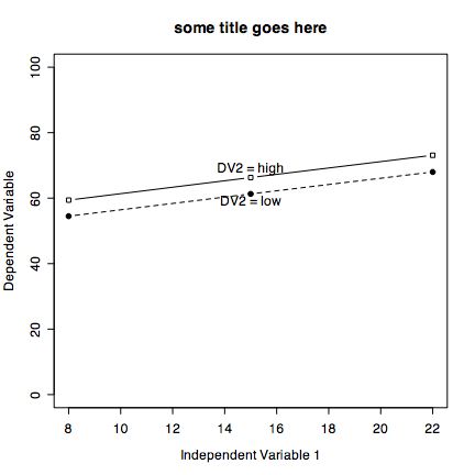
It is also easy to draw plots of specific points connected by lines. Consider if we have the experimental results on a Dependent Variable (DV) as a function of two Independent Variables (IV1 and IV2)
| IV 2 | ||
| Low | High | |
| IV 1 Low | 1 | 4 |
| IV 1 High | 3 | 2 |
iv2low=c(1,3)  #the Dependent variable values for low and high IV 1 and low IV2
iv2high=c(4,2) #the Dependent variable values for low and high IV 1 and high IV2

plot(iv2low,xlim=c(1,2),ylim=c(0,5),type="b", xlab="Independent Variable 1" ,ylab="Dependent Variable",  pch=19,main="some title")    #plot character is closed circle
points(iv2high, pch=22)    #plot characer is open square
lines(iv2high,lty="dashed")
text(1.2,1,"DV2 = low")    #change the location of these labels to fit the data
text(1.2,4,"DV2 = low")
Commands used in this tutorial
source("http://personality-project.org/r/useful.r")    #get some additional commands
install.packages("psych")      #just do this once
library("psych")     #do this everytime you start R

datafilename="Desktop/epi.big5.txt"     #name of data file


person.data =read.table(datafilename,header=TRUE)  #read the data file
#Alternatively, to read in a comma delimited file:
#data =read.table(datafilename,header=TRUE,sep=",")
summary(person.data)  #print out the min, max, range, mean, median, etc. of the data
round(mean(person.data),2)   #means of all variables, rounded to 2 decimals
round(sd(person.data),2)      #standard deviations, rounded to 2 decimals
describe(person.data)        #summary statistics
by(person.data,epilie<3,describe)   #summary statistics broken down by a categorical variable)
boxplot(person.data[1:5]) #show a boxplot of the first 5 variables

multi.hist(person.data)  #histograms of all the variables

round(cor(person.data,use="pairwise"),2)  #correlation matrix
pairs.panels(person.data[1:5])      #scatter plots, histograms,correlations

DV=performance   #The Dependent Variable
IV1=impulsivity  #continuous Independent Variable
IV2=time        #categorical Independent Variable

mydata=data.frame(DV,IV1,IV2)   #put them together into one data frame
attach(mydata)

zmydata=data.frame(scale(mydata))             #convert the data to standard scores to do the regression analysis
                                              #this makes the interaction term independent of the main effects
model=lm(DV~IV1+IV2+ IV1*IV2,data=zmydata)    #test the main effects of IV1 and IV2 and the interaction of IV1 and IV2
print(model)              #just show the coefficients
summary(model)            #show the coefficients as well as the probability estimates for the coefficients
attach(person.data)       #needed for the next command to work
by(person.data,time,function(x) summary(lm(performance~impulsivity,data=x))) #give the summary stats for the regression by location

par(mfrow=c(1,1))                      #set the graphics back to a 1 x 1 plot
symb=c(19,25,3,23)                     #choose some nice plotting symbols
colors=c("black","red","green","blue") #choose some nice colors

tod=as.integer(time < 10) +1          #I want a high and low time of day line -- time is actually 9 or 19, tod is now 1 or 2

plot(impulsivity,performance,pch=symb[tod],col=colors[tod],bg=colors[time],cex=1.0,main="Performance varies by time of day and impulsivity")   #show  the data points
by(person.data,time,function(x) abline(lm(performance~impulsivity,data=x)))  #show the best fitting regression for each group
text(6,60,"time=9 am")
text(6,90,"time= 7 pm ")


#show an interaction
iv2low=c(1,3)  #the Dependent variable values for low and high IV 1 and low IV2
iv2high=c(4,2) #the Dependent variable values for low and high IV 1 and low IV2

plot(iv2low,xlim=c(1,2),ylim=c(0,5),type="b", xlab="Independent Variable 1" ,ylab="Dependent Variable",  pch=19,main="some title")    #plot character is closed circle
points(iv2high, pch=22)    #plot characer is open square
lines(iv2high,lty="dashed")
text(1.2,1,"DV2 = low")    #change the location of these lables to fit the data
text(1.2,4,"DV2 = low")
Version of July 1, 2023