This page discusses the analysis and also shows how the analyses were done using the R computer package. For more details on using R, consult the very short tutorial or the more complete tutorial.
Before examining the recognition of true and false memories, we examined the effect of several variables upon the probability of recalling a true word. The first analysis is merely descriptive. Does recall show the normal serial position effect? How does the probability of false recall compare to the probability of real recall?
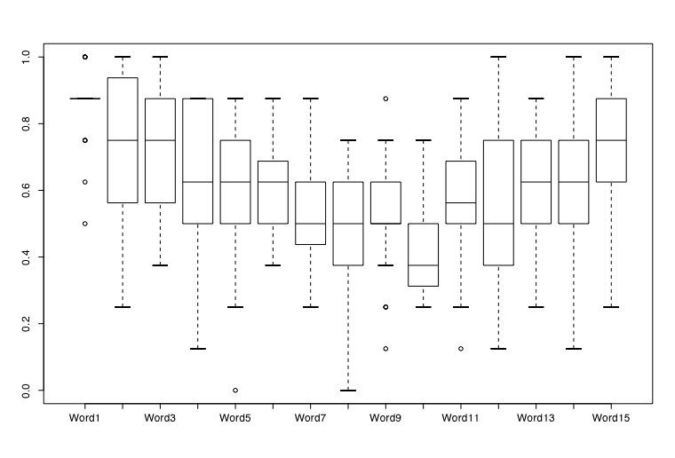
The data were transferred from the scoring sheets into a spreadsheet. These data were then read into R by using the read.clipboard() function. Two descriptive graphs were made: a boxplot of the 15 words which shows the variability of the subjects' data, as well as a more conventional plot of the means.
The raw data

Word1	Word2	Word3	Word4	Word5	Word6	Word7	Word8	Word9	Word10	Word11	Word12	Word13	Word14	Word15
8	7	8	4	7	5	4	3	4	4	5	3	4	4	6
7	6	7	4	6	5	4	3	4	4	5	7	5	4	7
7	6	8	5	6	5	5	6	6	3	5	6	6	7	7
7	5	6	6	6	7	4	4	5	5	6	5	5	3	5
8	7	8	6	3	6	2	4	4	3	2	1	2	7	8
7	8	5	4	6	4	3	3	5	4	6	3	6	6	5
8	8	5	5	2	7	5	4	4	6	4	3	6	6	5
8	2	4	1	4	3	3	3	5	3	4	1	6	3	7
7	6	7	5	5	4	5	5	4	4	2	5	5	5	5
6	5	4	6	5	5	3	4	2	2	2	3	3	5	6
7	8	7	7	6	3	4	5	6	3	5	7	5	5	3
6	4	5	2	3	5	4	0	2	3	4	3	4	6	5
8	8	7	7	4	5	4	3	7	2	7	4	6	6	6
5	4	5	3	0	6	5	3	2	2	4	5	5	4	8
7	6	5	4	4	3	4	5	5	5	5	4	7	5	7
7	4	4	7	4	5	4	4	3	4	4	6	5	6	8
7	8	7	7	5	5	4	4	6	5	6	5	5	6	4
7	8	6	7	7	3	4	5	4	4	1	6	3	4	4
7	7	7	7	4	6	4	3	5	6	5	6	6	4	5
7	4	7	7	3	6	7	6	4	2	6	8	7	8	6
6	5	3	3	4	5	3	4	1	2	4	3	2	1	2
7	7	8	6	5	4	5	5	4	2	6	2	5	6	6
4	3	4	4	6	4	3	2	4	3	4	2	2	3	7
7	7	4	5	5	5	5	3	5	3	4	2	4	4	7
To just copy these data into R, we can read from the clipboard. Unfortunately, until version 2.1.0 comes out, this command is different for PCs and Macs. But to get around this, I have created the "read.clipboard()" function. This may be obtained from the web by using the source command:
source("http://personality-project.org/r/useful.r") #useful additions to r
#now copy the data into the clipboard and read the clipboard
recall.words <- read.clipboard() #reads the data
recall.words <- recall.words/8 #convert to probabilities of recall
recall.words #echos the data to the console
boxplot(recall.words) #a boxplot of the results
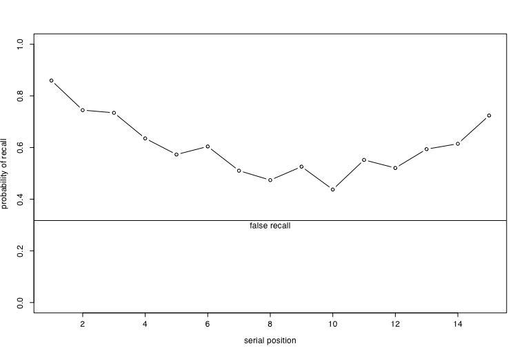
plot(recall.words,type="b",ylim=c(0,1),xlab = "serial position", ylab ="probability of recall")
abline(h=2.54/8) #a horizontal line for the false recalls
text(8,.3,"false recall") #add a label to the graph
results in the boxplot and the more conventional graphic
These two graphs suggest that normal memory processes were involved while subjects were learning the 16 lists. Words at the beginning and end of each list were much more likely to be recalled than were words in the middle of the list. False memories were recalled about 32% of the time.
To do this required entering the data into a data sheet and then reading it into the R system.
The first data set to read is the recall data for a few specific locations (1, 8 and 10) on each list. The variable labels reflect the condition of 2 or 3 seconds of study time and 45 or 90 seconds of recall time. Not in R, I combined the two replications for each subject for each condition.
r24	r34	r29	r39
3	4	5	4
2	5	5	4
3	4	4	3
4	5	5	2
2	4	5	5
2	2	1	3
2	3	4	5
3	6	3	3
3	4	4	3
2	3	4	2
4	3	2	5
4	3	5	4
3	4	3	4
3	3	4	4
4	5	4	5
4	3	1	3
4	2	3	5
3	0	3	5
4	4	4	4
3	4	3	6
1	3	4	6
3	5	4	3
2	2	4	3
#now copy the data into the clipboard and read the clipboard
recall <- read.clipboard()  #reads the data
recall                      #echos the data to the console


#produces this output

 recall
   r24 r34 r29 r39
1    3   4   5   4
2    2   5   5   4
...
21   1   3   4   6
22   3   5   4   3
23   2   2   4   3
These are the number of words recalled (6 maximum) in the 2 second or 3 second study trials and the 45 or 90 second recall trials. To convert these raw numbers to probability of recall, we can divide them all by 6.
recall <- recall/6 #the numbers now range from 0 to 1 to reflect the probability of recall.
We can examine whether there is an effect or study and recall interval by doing an analysis of variance. This allows us to ask the inferential question about how much of the variance of the Dependent Variable is associated with our manipulations of the Independent Variables. We ask the question of how likely is it to observe this much variation due to the IVs if there is in fact no effect of the IVs in the population. We are interested in the means for our conditions as well as the variance between means compared to the variance within subjects.
The analysis we will do is a complete within subject analysis which requires some manipulation of the data to put it into a form for an anova. ANOVA is done as a linear model (regression) of the IVs against the DV. With repeated measures, subjects becomes a variable and we string out the 23 * 4 array into a single vector of 92 values. We use the stack function to do this. Then we add values for the IVs, including the subject as an IV. We put the entire set into a "dataframe".
(Believe it or not, this is actually simpler than it seems at first glance. The dataframe can be thought of as a number of rows and columns where we need to define what goes into each column. Column 1 is simply the data for each subject, strung out into 1 long column. Column 2 gives us the variable names from the original data. Column 3 (study) is either "short" or "long". It is made up by repeating the names "short" and "long" numcases (23) times each. Because this does not fill up the column, this pattern is then repeated until it does. Column 4 (time) does the same thing but puts in "45" or "90" 2 * numcases times each. It also doesn't fill up the column and so automatically repeats until it does. Finally, the last column gives labels to each subject. These labels are then repeated 4 times.)
#set a few general variables

numcases <- 23     #how many subjects
numlevelsvar1  <- 2  #how many levels of variable 1?
numlevelsvar2  <- 2  #how many levels of variable 2?

numvar <- numlevelsvar1 * numlevelsvar2  #figure out the number of variables
stackeddata <- stack(recall)     #strings out the data into 1 column

#create a dataframe with the DVs followed by the IVs
data.df <- data.frame(stackeddata,
    study = factor(rep(c("short","long"),c(numcases,numcases))),
    time = factor(rep(c("45","90"),c(numlevels1*numcases,numlevels1*numcases))),
    subj = factor(rep(paste("subj",1:numcases, sep=""), numvar))
   )
The original data were
  recall
    r24  r34  r29  r39
1  0.50 0.67 0.83 0.67
2  0.33 0.83 0.83 0.67
...
22 0.50 0.83 0.67 0.50
23 0.33 0.33 0.67 0.50


The "stacked" data with the variable values added are


     values ind study time   subj
1  0.5000000 r24 short   45  subj1
2  0.3333333 r24 short   45  subj2
...
22 0.5000000 r24 short   45 subj22
23 0.3333333 r24 short   45 subj23
24 0.6666667 r34  long   45  subj1
...
46 0.3333333 r34  long   45 subj23
47 0.8333333 r29 short   90  subj1
...
69 0.6666667 r29 short   90 subj23
70 0.6666667 r39  long   90  subj1
71 0.6666667 r39  long   90  subj2
...
91 0.5000000 r39  long   90 subj22
92 0.5000000 r39  long   90 subj23
Now that the data are in a useful form, we do the Analysis of Variance (ANOVA) with repeated measures.
recall.aov= aov(values ~ time * study + Error(subj/(time * study)), data=data.df)   #do the ANOVA
print(model.tables(recall.aov,"means"),digits=3)   #show the cell means for the anova table

summary(recall.aov)                                #show the output for ANOVA


Produces this output:

recall.aov= aov(values ~ time * study + Error(subj/(time * study)), data=data.df)   #do the ANOVA
 print(model.tables(recall.aov,"means"),digits=3)   #show the cell means for the anova table
Tables of means
Grand mean

0.5869565                <- overall probability of recall

 time
       45     90
     0.54  0.634       <- it seems as if more words were recalled in 90 than 45 seconds
rep 46.00 46.000

 study
      long  short
     0.623  0.551    <- and that longer study times helped later recall
rep 46.000 46.000

 time:study
     study
time  long  short
  45   0.59  0.49
  rep 23.00 23.00
  90   0.66  0.61
  rep 23.00 23.00
>
  #now  test these differences for statistical significance
  #that is, how likely would you observe these differences if the population means were identical?
> summary(recall.aov)                                #show the output

Error: subj
          Df  Sum Sq Mean Sq F value Pr(>F)        <- the within subject error term
Residuals 22 0.81824 0.03719

Error: subj:time
          Df  Sum Sq Mean Sq F value Pr(>F)
time       1 0.20411 0.20411  5.3612 0.0303 *      <- the  effect of recall time has a "p value " of .03
Residuals 22 0.83756 0.03807
---
Signif. codes:  0 `***' 0.001 `**' 0.01 `*' 0.05 `.' 0.1 ` ' 1

Error: subj:study
          Df  Sum Sq Mean Sq F value  Pr(>F)
study      1 0.12077 0.12077  5.9219 0.02353 *   <- the effect of study time has a "p value" of .02
Residuals 22 0.44867 0.02039
---
Signif. codes:  0 `***' 0.001 `**' 0.01 `*' 0.05 `.' 0.1 ` ' 1

Error: subj:time:study
           Df  Sum Sq Mean Sq F value Pr(>F)
time:study  1 0.01087 0.01087   0.232 0.6348
Residuals  22 1.03080 0.04685
Here are all the commands grouped together:
source("http://personality-project.org/r/useful.r")   #get some useful additions

#now copy the data into the clipboard and read the clipboard
recall <- read.clipboard()  #reads the data
recall                      #echos the data
recall <- recall/6          #convert to probability of recall
#set a few general variables
numcases <- 23     #how many subjects
numlevelsvar1  <- 2  #how many levels of variable 1?
numlevelsvar2  <- 2  #how many levels of variable 2?
numvar <- numlevelsvar1 * numlevelsvar2
stackeddata <- stack(recall)     #strings out the data into 1 column

#create a dataframe with the DVs followed by the IVs
data.df <- data.frame(stackeddata,
    study = factor(rep(c("short","long"),c(numcases,numcases))),
    time = factor(rep(c("45","90"),c(numlevels1*numcases,numlevels1*numcases))),
    subj = factor(rep(paste("subj",1:numcases, sep=""), numvar))
   )

recall.aov= aov(values ~ time * study + Error(subj/(time * study)), data=data.df)   #do the ANOVA

print(model.tables(recall.aov,"means"),digits=3)   #show the cell means for the anova table

summary(recall.aov)                                #show the output for ANOVA
More than just examining recall, we were interested in the effect of our manipulations on recognition of words that were presented (True memories) and high associate words that were not presented (False memories). In addition, we were interested in whether recognition for True and False memories are affected by study time (2 vs 3 seconds) and recall interval (45 vs. 90). We were also interested in whether having a chance to recall (Math vs. Recall) makes a difference. This is a complicated analysis and we will build up to it by doing a number of simpler analyses first. In fact, the ANOVA was developed for just this case. It allows us to examine many effects at the same time, from broad main effects to complex interactions between variables.
The raw data are the number of words correctly and incorrectly recognized on the recognition sheet depending upon conditions. The variable labels are an attempt at specifying conditions (e.g., r vs f for real versus false, 0 or 1 for no recall (math) vs recall, 2 vs 3 for 2 versus 3 seconds of study, and 4 vs 9 for 45 versus 9 seconds recall interval).
Before doing any analyses, we will need to rescale the numbers to put them on a 0 - 1 scale. The reall numbers range from 0-6 and the false from 0-2. We can do this by dividing the recognition matrix by a vector of 6s and 2s. Then we need to stack the data and create a data frame with the appropriate conditions.
   r024 r029 r034 r039 r124 r129 r134 r139 f024 f029 f034 f039 f124 f129 f134 f139
1     5    4    6    4    4    6    6    5    1    1    2    2    1    0    1    2
2     5    5    3    4    5    5    6    5    0    0    1    0    1    1    0    0
3     5    1    4    6    6    6    6    4    0    0    0    1    1    1    0    0
4     6    3    6    3    4    5    5    3    1    2    2    1    2    1    2    0
5     6    0    5    5    3    4    5    5    1    1    2    0    1    1    0    0
6     0    0    1    3    3    3    3    4    0    0    1    1    1    2    1    2
7     5    4    6    5    3    5    5    5    1    2    2    1    2    1    1    2
8     5    4    4    5    5    5    6    3    0    0    0    0    1    0    1    1
9     3    3    5    4    5    5    6    5    0    0    0    0    1    1    0    0
10    5    2    4    6    3    5    5    3    1    2    2    2    2    2    2    1
11    2    5    6    6    5    3    6    6    1    1    1    0    0    1    1    1
12    3    3    6    1    5    4    6    6    0    0    0    0    1    2    1    1
13    5    5    4    5    4    4    5    5    2    1    1    1    0    0    1    1
14    5    6    5    5    5    6    6    6    1    0    1    1    1    1    1    2
15    6    5    6    4    6    5    6    6    2    1    1    0    0    0    1    0
16    3    6    6    3    6    2    6    4    0    0    1    1    0    1    0    1
17    6    5    6    4    5    6    5    4    2    0    2    1    1    1    2    1
18    3    5    6    4    6    5    3    5    1    2    2    1    1    2    1    2
19    5    6    6    4    6    6    6    6    2    0    1    1    1    1    0    1
20    1    0    0    0    2    2    5    5    1    1    1    1    2    0    0    1
21    2    3    6    2    3    6    4    6    1    0    2    1    1    2    2    2
22    5    6    6    4    6    5    6    4    2    1    2    2    1    1    1    0
23    2    5    3    4    1    5    4    4    0    0    0    0    1    1    1    0


#Copy these to the clipboard and then read the clipboard:
recognition <- read.clipboard()
recognition[,1:8] <- recognition[,1:8]/6  #divide the first 8 by 6, the last 8 by 2
recognition[9:16]<-recognition[,9:16]/2


#set a few general variables
numcases <- 23     #how many subjects
numlevelsvar1  <- 2  #how many levels of variable 1?
numlevelsvar2  <- 2  #how many levels of variable 2?
numlevelsvar3  <- 2  #how many levels of variable 3?
numlevelsvar4  <- 2  #how many levels of variable 4?

numvar <- numlevelsvar1 * numlevelsvar2 * numlevelsvar3 * numlevelsvar4

stackeddata <- stack(recognition)   # string out into a 16*23 long vector

#create a dataframe with the DVs followed by the IVs
data.df <- data.frame(stackeddata,
    wordtype = factor(rep(c("real","false"),c(numvar*numcases/2,numvar*numcases/2))),
    recall = factor(rep(c("math","recall"),c(numcases*numlevels1*numlevels2,numcases*numlevels1*numlevels2))),
    study = factor(rep(c("short","long"),c(numcases*numlevels1,numcases*numlevels1))),
    time = factor(rep(c("45","90"),c(numcases,numcases))),
    subj = factor(rep(paste("subj",1:numcases, sep=""), numvar))
   )

recog.aov= aov(values ~ wordtype* recall* time * study + Error(subj/(wordtype*recall*time * study)), data=data.df)   #do the ANOVA

print(model.tables(recog.aov,"means"),digits=3)   #show the cell means for the anova table

summary(recog.aov)                                #show the output for ANOVA
This produces pages of output, first of the means, organized by the various combinations of the independent variables, and then the actual inferential tests using ANOVA.
Tables of means
Grand mean         What is the overall mean probability of recognition?

0.5978261

 wordtype         Real words are recognized more than false words
      false    real
      0.454   0.742
rep 184.000 184.000      rep (or replications) is how many observations went into this mean

 recall          more words were recognized if given a chance to recall
       math  recall
      0.562   0.634
rep 184.000 184.000

 time            more words were recognized after a shorter recall interval!
        45      90
      0.63   0.566
rep 184.00 184.000

 study           longer times (3 seconds vs. 2 secs) lead to better recognition
       long   short
      0.624   0.572
rep 184.000 184.000

 wordtype:recall
        recall
wordtype math recall
   false  0.4  0.5
   rep   92.0 92.0
   real   0.7  0.8
   rep   92.0 92.0

 wordtype:time
        time
wordtype 45   90
   false  0.5  0.4
   rep   92.0 92.0
   real   0.8  0.7
   rep   92.0 92.0

 recall:time    longer time doing math seemed to reduce later recognition
        time
recall   45   90
  math    0.6  0.5
  rep    92.0 92.0
  recall  0.6  0.6
  rep    92.0 92.0

 wordtype:study
        study
wordtype long short
   false  0.5  0.4
   rep   92.0 92.0
   real   0.8  0.7
   rep   92.0 92.0

 recall:study
        study
recall   long short
  math    0.6  0.5
  rep    92.0 92.0
  recall  0.6  0.6
  rep    92.0 92.0

 time:study
     study
time  long short
  45   0.7  0.6
  rep 92.0 92.0
  90   0.6  0.6
  rep 92.0 92.0

 wordtype:recall:time
, , time = 45

        recall
wordtype math recall
   false  0.5  0.5
   rep   46.0 46.0
   real   0.7  0.8
   rep   46.0 46.0

, , time = 90

        recall
wordtype math recall
   false  0.4  0.5
   rep   46.0 46.0
   real   0.6  0.8
   rep   46.0 46.0


 wordtype:recall:study
, , study = long

        recall
wordtype math recall
   false  0.5  0.4
   rep   46.0 46.0
   real   0.7  0.8
   rep   46.0 46.0

, , study = short

        recall
wordtype math recall
   false  0.4  0.5
   rep   46.0 46.0
   real   0.6  0.8
   rep   46.0 46.0


 wordtype:time:study
, , study = long

        time
wordtype 45   90
   false  0.5  0.4
   rep   46.0 46.0
   real   0.8  0.7
   rep   46.0 46.0

, , study = short

        time
wordtype 45   90
   false  0.5  0.4
   rep   46.0 46.0
   real   0.7  0.7
   rep   46.0 46.0


 recall:time:study
, , study = long

        time
recall   45   90
  math    0.7  0.5
  rep    46.0 46.0
  recall  0.7  0.6
  rep    46.0 46.0

, , study = short

        time
recall   45   90
  math    0.6  0.5
  rep    46.0 46.0
  recall  0.6  0.6
  rep    46.0 46.0


 wordtype:recall:time:study
, , time = 45, study = long

        recall
wordtype math  recall
   false  0.59  0.43
   rep   23.00 23.00
   real   0.80  0.88
   rep   23.00 23.00

, , time = 90, study = long

        recall
wordtype math  recall
   false  0.39  0.46
   rep   23.00 23.00
   real   0.66  0.79
   rep   23.00 23.00

, , time = 45, study = short

        recall
wordtype math  recall
   false  0.43  0.50
   rep   23.00 23.00
   real   0.67  0.73
   rep   23.00 23.00

, , time = 90, study = short

        recall
wordtype math  recall
   false  0.33  0.50
   rep   23.00 23.00
   real   0.62  0.78
   rep   23.00 23.00
After all of these means, we want to think about which make the most difference. That is to say, some of these differences are what we would expect by chance. Lets look at the ANOVA output to see which means are most important to think about. Each ANOVA table reports a number of different things.
Analysis of Variance summary table:


Error: subj
          Df Sum Sq Mean Sq F value Pr(>F)
Residuals 22 6.3741  0.2897

Error: subj:wordtype
          Df Sum Sq Mean Sq F value    Pr(>F)
wordtype   1 7.6332  7.6332  27.268 3.084e-05 ***
Residuals 22 6.1585  0.2799
---
Signif. codes:  0 `***' 0.001 `**' 0.01 `*' 0.05 `.' 0.1 ` ' 1

Error: subj:recall
          Df Sum Sq Mean Sq F value  Pr(>F)
recall     1 0.4831  0.4831  3.2326 0.08592 .
Residuals 22 3.2877  0.1494
---
Signif. codes:  0 `***' 0.001 `**' 0.01 `*' 0.05 `.' 0.1 ` ' 1

Error: subj:time
          Df  Sum Sq Mean Sq F value  Pr(>F)
time       1 0.36987 0.36987  5.1003 0.03418 *
Residuals 22 1.59541 0.07252
---
Signif. codes:  0 `***' 0.001 `**' 0.01 `*' 0.05 `.' 0.1 ` ' 1

Error: subj:study
          Df  Sum Sq Mean Sq F value  Pr(>F)
study      1 0.25393 0.25393  4.8921 0.03767 *
Residuals 22 1.14191 0.05190
---
Signif. codes:  0 `***' 0.001 `**' 0.01 `*' 0.05 `.' 0.1 ` ' 1

Error: subj:wordtype:recall
                Df Sum Sq Mean Sq F value Pr(>F)
wordtype:recall  1 0.1090  0.1090  1.4993 0.2337
Residuals       22 1.5993  0.0727

Error: subj:wordtype:time
              Df  Sum Sq Mean Sq F value Pr(>F)
wordtype:time  1 0.00483 0.00483  0.0998  0.755
Residuals     22 1.06461 0.04839

Error: subj:recall:time
            Df  Sum Sq Mean Sq F value  Pr(>F)
recall:time  1 0.32880 0.32880   5.379 0.03006 *
Residuals   22 1.34481 0.06113
---
Signif. codes:  0 `***' 0.001 `**' 0.01 `*' 0.05 `.' 0.1 ` ' 1

Error: subj:wordtype:study
               Df  Sum Sq Mean Sq F value Pr(>F)
wordtype:study  1 0.05918 0.05918  0.9305 0.3452
Residuals      22 1.39915 0.06360

Error: subj:recall:study
             Df  Sum Sq Mean Sq F value Pr(>F)
recall:study  1 0.15972 0.15972  2.3211 0.1419
Residuals    22 1.51389 0.06881

Error: subj:time:study
           Df  Sum Sq Mean Sq F value Pr(>F)
time:study  1 0.12077 0.12077  2.1542 0.1563
Residuals  22 1.23339 0.05606

Error: subj:wordtype:recall:time
                     Df  Sum Sq Mean Sq F value Pr(>F)
wordtype:recall:time  1 0.04348 0.04348  0.7037 0.4106
Residuals            22 1.35930 0.06179

Error: subj:wordtype:recall:study
                      Df  Sum Sq Mean Sq F value  Pr(>F)
wordtype:recall:study  1 0.14614 0.14614  3.0668 0.09384 .
Residuals             22 1.04831 0.04765
---
Signif. codes:  0 `***' 0.001 `**' 0.01 `*' 0.05 `.' 0.1 ` ' 1

Error: subj:wordtype:time:study
                    Df  Sum Sq Mean Sq F value Pr(>F)
wordtype:time:study  1 0.03653 0.03653  0.6404 0.4321
Residuals           22 1.25513 0.05705

Error: subj:recall:time:study
                  Df  Sum Sq Mean Sq F value Pr(>F)
recall:time:study  1 0.00483 0.00483  0.0804 0.7794
Residuals         22 1.32156 0.06007

Error: subj:wordtype:recall:time:study
                           Df  Sum Sq Mean Sq F value Pr(>F)
wordtype:recall:time:study  1 0.03653 0.03653  0.4152  0.526
Residuals                  22 1.93569 0.08799
From the ANOVA table we can see that there are 3 main effects and one interaction that are worth discussing: Word type (real or false), recall time (45 vs. 90) and study time (2 vs 3). In addition, recall vs. math interacted with recall time. Note that real versus false did not interact with anything, suggesting that the process of retrieving "real" memories and "false" memories do not differ.