Two alternative estimates of reliability that take into account the hierarchical structure of the inventory are McDonald’s ωh and ωt (McDonald, 1999). These may be found in R in one step using one of two functions in the psych package: the omega function for an exploratory analysis (See Figure 1) or omegaSem for a confirmatory analysis using the sem package solution based upon the exploratory solution from omega. This guide explains how to do it for the non or novice R user. These set of instructions are adapted from three different sets of notes that the interested reader might find helpful: A set of slides developed for a two hour short course in R given in May, 2012 to the Association of Psychological Science http://personality-project.org/r/aps/aps-short.pdf as well as a short guide to R http://personality-project.org/r/ for psychologists and the vignette for the psych package http://cran.r-project.org/web/packages/psych/vignettes/overview.pdf.
McDonald has proposed coefficient omega (hierarchical) (ωh) as an estimate of the general factor saturation of a test. Zinbarg et al. (2005) http://personality-project.org/revelle/publications/zinbarg.revelle.pmet.05.pdf compare McDonald’s ωh to Cronbach’s α and Revelle’s β. They conclude that ωh is the best estimate. (See also Zinbarg et al. (2006) and Revelle and Zinbarg (2009) http://personality-project.org/revelle/publications/revelle.zinbarg.08.pdf ).
One way to find ωh is to do a factor analysis of the original data set, rotate the factors obliquely, factor that correlation matrix, do a Schmid-Leiman (schmid) transformation to find general factor loadings, and then find ωh. This is done using the omega function in the psych package in R. This requires installing and using both R as well as the psych package (Revelle, 2013).
Assuming that your data are in a file called my.data, and that you have the necessary packages installed, to find ωh requires two lines of code:
The resulting output will be both graphical (see Figure 1) and textual.
This guide helps the naive R user to issue those two lines.
To find ωh in R obviously requires installing R on your computer. This is very easy to do (see section 2.1.1) and needs to be done once.
The power of R is in the supplemental packages. At a minimum, you will need to install three package (psych (Revelle, 2013), GPArotation (Bernaards and Jennrich, 2005) and MASS (Venables and Ripley, 2002). With these three packages, you will be be able to find ωh using Exploratory Factor Analysis. If you want to find it using Confirmatory Factor Analysis, you will also need to add the sem (Fox et al., 2013) and matrixcalc (Novomestky, 2012) packages. For a more complete installation of a number of psychometric packages, you can install and activate a package (ctv) that installs a large set of psychometrically relevant packages. As is true for R, you will need to install packages just once.
install.packages(c("psych","GPArotation","MASS","sem","matrixcalc"))
First go to the Comprehensive R Archive Network (CRAN) at http://cran.r-project.org: (Figure 2)

Choose your operating system and then download and install the appropriate version
For a PC: (Figure 3)
Download and install the appropriate version – PC
For a Mac: download and install the appropriate version – Mac (Figure 5)

Starting R on a PC
Start up R and get ready to play (Mac version)
Once R is installed on your machine, you still need to install a few relevant “packages”. Packages are what make R so powerful, for they are special sets of functions that are designed for one particular application. In the case of the psych package, that application is for doing the kind of basic data analysis and psychometric analysis that personality psychologists find particularly useful.
You may either install the minimum set of packages necessary to do the analysis using an EFA approach (recommended) or a few more packages to do both the EFA and a CFA approach. It is also possible to add many psychometrically relevant packages all at once by using the “task views” approach.
Install the sem package as well
Install all the psychometric packages from the “psychometrics” task view.
You are almost ready. But first you need to make the psych package active. You only need to do this once per session.
You are almost there. But first you need to read in your data from your data file.
There are of course many ways to enter data into R. Reading from a local file using read.table is perhaps the most preferred. You first need to find the file and then read it. This can be done with the file.choose and read.table functions:
file.choose opens a search window on your system just like any open file command does. It doesn’t actually read the file, it just finds the file. The read command is also necessary.
However, many users will enter their data in a text editor or spreadsheet program and then want to copy and paste into R. This may be done by using read.table and specifying the input file as “clipboard" (PCs) or “pipe(pbpaste)" (Macs). Alternatively, the read.clipboard set of functions are perhaps more user friendly:
For example, given a data set copied to the clipboard from a spreadsheet, just enter the command
This will work if every data field has a value and even missing data are given some values (e.g., NA or -999). If the data were entered in a spreadsheet and the missing values were just empty cells, then the data should be read in as a tab delimited or by using the read.clipboard.tab function.
For the case of data in fixed width fields (some old data sets tend to have this format), copy to the clipboard and then specify the width of each field (in the example below, the first variable is 5 columns, the second is 2 columns, the next 5 are 1 column the last 4 are 3 columns).
To read data from an SPSS, SAS, or Systat file, you must use the foreign package. This might need to be installed (see 2.1.2 for instructions for installing packages).
read.spss reads a file stored by the SPSS save or export commands.
An example of reading from an SPSS file and then describing the data set to make it looks ok.
Although you probably want to jump right in and find ω, you should first make sure that your data are reasonable. Use the describe function to get some basic descriptive statistics. This next example takes advantage of a built in data set.
There are, of course, all kinds of things you could do with your data at this point, but read about them in the vignette for the psych package http://cran.r-project.org/web/packages/psych/vignettes/overview.pdf.
Two alternative estimates of reliability that take into account the hierarchical structure of the inventory are McDonald’s ωh and ωt. These may be found using the omega function for an exploratory analysis (See Figure 1) or omegaSem for a confirmatory analysis using the sem based upon the exploratory solution from omega.
McDonald (1999) has proposed coefficient omega (hierarchical) (ωh) as an estimate of the general factor saturation of a test. Zinbarg et al. (2005) http://personality-project.org/revelle/publications/zinbarg.revelle.pmet.05.pdf compare McDonald’s ωh to Cronbach’s α and Revelle’s β. They conclude that ωh is the best estimate. (See also Zinbarg et al. (2006) and Revelle and Zinbarg (2009) http://personality-project.org/revelle/publications/revelle.zinbarg.08.pdf ).
One way to find ωh is to do a factor analysis of the original data set, rotate the factors obliquely, factor that correlation matrix, do a Schmid-Leiman (schmid) transformation to find general factor loadings, and then find ωh.
ωh differs slightly as a function of how the factors are estimated. Three options are available, the default will do a minimum residual factor analysis, fm=“pa" does a principal axes factor analysis (factor.pa), and fm=“mle" provides a maximum likelihood solution.
For ability items, it is typically the case that all items will have positive loadings on the general factor. However, for non-cognitive items it is frequently the case that some items are to be scored positively, and some negatively. Although probably better to specify which directions the items are to be scored by specifying a key vector, if flip =TRUE (the default), items will be reversed so that they have positive loadings on the general factor. The keys are reported so that scores can be found using the score.items function. Arbitrarily reversing items this way can overestimate the general factor. (See the example with a simulated circumplex).
β, an alternative to ω, is defined as the worst split half reliability. It can be estimated by using iclust (Item Cluster analysis: a hierarchical clustering algorithm). For a very complimentary review of why the iclust algorithm is useful in scale construction, see Cooksey and Soutar (2006).
The omega function uses exploratory factor analysis to estimate the ωh coefficient. It is important to remember that “A recommendation that should be heeded, regardless of the method chosen to estimate ωh, is to always examine the pattern of the estimated general factor loadings prior to estimating ωh. Such an examination constitutes an informal test of the assumption that there is a latent variable common to all of the scale’s indicators that can be conducted even in the context of EFA. If the loadings were salient for only a relatively small subset of the indicators, this would suggest that there is no true general factor underlying the covariance matrix. Just such an informal assumption test would have afforded a great deal of protection against the possibility of misinterpreting the misleading ωh estimates occasionally produced in the simulations reported here." (Zinbarg et al., 2006, p 137).
Although ωh is uniquely defined only for cases where 3 or more subfactors are extracted, it is sometimes desired to have a two factor solution. By default this is done by forcing the schmid extraction to treat the two subfactors as having equal loadings.
There are three possible options for this condition: setting the general factor loadings
between the two lower order factors to be “equal" which will be the  where rab is the
oblique correlation between the factors) or to “first" or “second" in which case the
general factor is equated with either the first or second group factor. A message is issued
suggesting that the model is not really well defined. This solution discussed in Zinbarg
et al., 2007. To do this in omega, add the option=“first" or option=“second" to the
call.
where rab is the
oblique correlation between the factors) or to “first" or “second" in which case the
general factor is equated with either the first or second group factor. A message is issued
suggesting that the model is not really well defined. This solution discussed in Zinbarg
et al., 2007. To do this in omega, add the option=“first" or option=“second" to the
call.
Although obviously not meaningful for a 1 factor solution, it is of course possible to find the sum of the loadings on the first (and only) factor, square them, and compare them to the overall matrix variance. This is done, with appropriate complaints.
In addition to ωh, another of McDonald’s coefficients is ωt. This is an estimate of the total reliability of a test.
McDonald’s ωt, which is similar to Guttman’s λ6, (see guttman) uses the estimates of uniqueness
u2 from factor analysis to find ej2. This is based on a decomposition of the variance of a test
score, Vx into four parts: that due to a general factor,  , that due to a set of group factors,
  ,
(factors common to some but not all of the items), specific factors,
,
(factors common to some but not all of the items), specific factors,  unique to each
item, and
unique to each
item, and  , random error. (Because specific variance can not be distinguished from
random error unless the test is given at least twice, some combine these both into
error).
, random error. (Because specific variance can not be distinguished from
random error unless the test is given at least twice, some combine these both into
error).
Letting  =
=  +
+ +
+ +
+ then the communality of itemj, based upon general as well as group
factors, hj2 = cj2 +∑fij2 and the unique variance for the item uj2 = σj2(1-hj2) may
be used to estimate the test reliability. That is, if hj2 is the communality of itemj,
based upon general as well as group factors, then for standardized items, ej2 = 1-hj2
and
then the communality of itemj, based upon general as well as group
factors, hj2 = cj2 +∑fij2 and the unique variance for the item uj2 = σj2(1-hj2) may
be used to estimate the test reliability. That is, if hj2 is the communality of itemj,
based upon general as well as group factors, then for standardized items, ej2 = 1-hj2
and
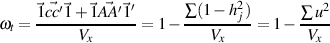
It is important to distinguish here between the two ω coefficients of McDonald, 1978 and Equation 6.20a of McDonald, 1999, ωt and ωh. While the former is based upon the sum of squared loadings on all the factors, the latter is based upon the sum of the squared loadings on the general factor.

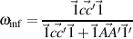
Another estimate reported is the omega for an infinite length test with a structure similar to the observed test. This is found by
It can be shown In the case of simulated variables, that the amount of variance attributable to a general factor (ωh) is quite large, and the reliability of the set of items is somewhat greater than that estimated by α or λ6.
Just call it. For the next example, we find ω for a data set from Thurstone. To find it for your data, replace Thurstone with my.data.
The omegaSem function will do an exploratory analysis and then take the highest loading items on each factor and do a confirmatory factor analysis using the sem package. These results can produce slightly different estimates of ωh, primarily because cross loadings are modeled as part of the general factor.
Bernaards, C. and Jennrich, R. (2005). Gradient projection algorithms and software for arbitrary rotation criteria in factor analysis. Educational and Psychological Measurement, 65(5):676.
Cooksey, R. and Soutar, G. (2006). Coefficient beta and hierarchical item clustering - an analytical procedure for establishing and displaying the dimensionality and homogeneity of summated scales. Organizational Research Methods, 9:78–98.
Fox, J., Nie, Z., and Byrnes, J. (2013). sem: Structural Equation Models. R package version 3.1-0.
McDonald, R. P. (1999). Test theory: A unified treatment. L. Erlbaum Associates, Mahwah, N.J.
Novomestky, F. (2012). matrixcalc: Collection of functions for matrix calculations. R package version 1.0-3.
Revelle, W. (2013). psych: Procedures for Personality and Psychological Research. Northwestern University, Evanston, http://cran.r-project.org/web/packages/psych/. R package version 1.3.2.
Revelle, W. and Zinbarg, R. E. (2009). Coefficients alpha, beta, omega and the glb: comments on Sijtsma. Psychometrika, 74(1):145–154.
Venables, W. N. and Ripley, B. D. (2002). Modern Applied Statistics with S. Springer, New York, fourth edition. ISBN 0-387-95457-0.
Zinbarg, R. E., Revelle, W., Yovel, I., and Li, W. (2005). Cronbach’s α, Revelle’s β, and McDonald’s ωH): Their relations with each other and two alternative conceptualizations of reliability. Psychometrika, 70(1):123–133.
Zinbarg, R. E., Yovel, I., Revelle, W., and McDonald, R. P. (2006). Estimating generalizability to a latent variable common to all of a scale’s indicators: A comparison of estimators for ωh. Applied Psychological Measurement, 30(2):121–144.


