Simulations of distributions
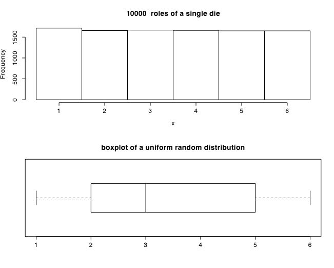
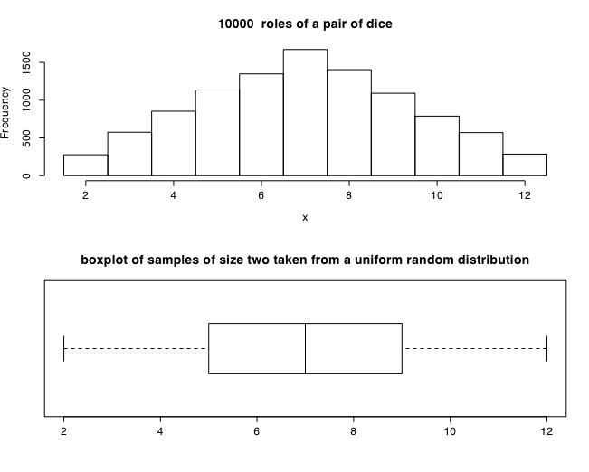
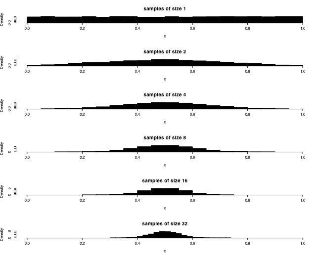
The following examples use the R stats program to show this graphically. The first example uses a uniform (rectangular) distribution. An example of this case is of a single die with the values of 1-6. The second example is of two dice with totals ranging from 2-12. Notice that although one die produces a rectangular distribution, two dice show a distribution peaking at 7. The next set of examples show the distribution of sample means for samples of size 1 .. 32 taken from a rectangular distribution.
This figure was produced using the following R code.
#distributions of a single six sided die
#generate a uniform random distribution from min to max

numcases <- 10000                           #how many cases to generate
min <- 1                                  #set parameters
max <- 6
x <- as.integer(runif(numcases,min,max+1) )        #generate random uniform numcases numbers from min to max
                                        #as.integer truncates, round converts to integers, add .5 for equal intervals
par(mfrow=c(2,1))                        #stack two figures above each other
hist(x,main=paste( numcases," roles of a single die"),breaks=seq(min-.5,max+.5,1))          #show the histogram
boxplot(x, horizontal=TRUE,range=1)              # and the boxplot
title("boxplot of a uniform random distribution")
#end of first demo
Distribution of two dice
Distribution of two dice. The sum of two dice is not rectangular, but is peaked at the middle (hint, how many ways can you get a 2, a 3, ... a 7, .. 12.).
The following R code produced this figure.
#generate a uniform random distribution from min to max for numcases samples of size 2
numcases <- 10000                            #how many cases to generate
min <- 0                                    #set parameters
max <- 6
x <- round(runif(numcases,min,max)+.5)+round(runif(numcases,min,max)+.5)
par(mfrow=c(2,1))                        #stack two figures above each other
hist(x,breaks=seq(1.5,12.5),main=paste( numcases," roles of a pair of dice"))          #show the histogram
boxplot(x, horizontal=TRUE,range=1)      # and the boxplot
title("boxplot of samples of size two taken from a uniform random distribution")

#end of second demo
Samples from a continuous uniform random distribution
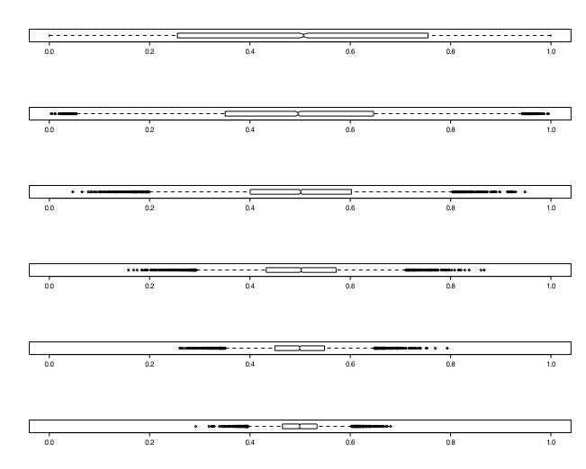
We can generalize the case of 1 or two dice to the case of samples of varying size taken from a continuous distribution ranging from 0-1. This next simulation shows the distribution of samples of sizes 1, 2, 4, ... 32 taken from a uniform distribution. Note, for each sample, we are finding the average value of the sample, rather than the sum as we were doing in the case of the dice.
##show distribution of sample means of varying size samples
numcases <- 10000 #how many samples to take?
min <- 0 #lowest value
max <- 1
ntimes <- 6
op<- par(mfrow=c(ntimes,1)) #stack ntimes graphs on top of each other
i2 <- 1 #initialize counters
for (i in 1:ntimes) #repeat n times
{ sample=rep(0,numcases) #create a vector
k=0 #start off with an empty set of counters
for (j in 1:i2) # inner loop
{
sample <- sample +runif(numcases,min,max)
k <- k+1 }
x <- sample/k
out <- c(k,mean(x),sd(x))
#print(out,digit=3)
hist(x, xlim=range(0,1),prob=T ,main=paste( "samples of size", k ),col="black")
i2 <- 2*i2
} #end of i loop
 #do the same thing, but this time show a boxplot
numcases <- 10000 #how many samples to take?
min <- 0 #lowest value
max <- 1
ntimes <- 6
par(mfrow=c(ntimes,1)) #stack ntimes graphs on top of each other
i2 <- 1 #initialize counters
for (i in 1:ntimes) #repeat 5 times
{ sample <- 0 ; k <- 0 #start off with an empty set of counters
for (j in 1:i2) # inner loop
{
sample <- sample +runif(numcases,min,max)
k <- k+1 }
x <- sample/k
out <- c(k,mean(x),sd(x))
boxplot(x, horizontal=TRUE, ylim=c(0,1), range=1,notch=T) # and the boxplot
i2 <- 2*i2}
#do the same thing, but this time show a boxplot
numcases <- 10000 #how many samples to take?
min <- 0 #lowest value
max <- 1
ntimes <- 6
par(mfrow=c(ntimes,1)) #stack ntimes graphs on top of each other
i2 <- 1 #initialize counters
for (i in 1:ntimes) #repeat 5 times
{ sample <- 0 ; k <- 0 #start off with an empty set of counters
for (j in 1:i2) # inner loop
{
sample <- sample +runif(numcases,min,max)
k <- k+1 }
x <- sample/k
out <- c(k,mean(x),sd(x))
boxplot(x, horizontal=TRUE, ylim=c(0,1), range=1,notch=T) # and the boxplot
i2 <- 2*i2}
 #Demonstration of the effect of sample size on distributions
#each sample is then replicated numcases times
filename <- "distributions2.pdf"
pdf(filename,width=6, height=9)
numcases <- 10000 #how many samples to take?
min <- 0 #lowest value
max <- 1
ntimes <- 3
par(mfrow=c(2*ntimes,1)) #stack ntimes graphs on top of each other
i2 <- 1 #initialize counters
for (i in 1:ntimes) #repeat 5 times
{ sample <- 0 ; k <- 0 #start off with an empty set of counters
for (j in 1:i2) # inner loop
{
sample <- sample +runif(numcases,min,max)
k <- k+1 }
x <- sample/k
out <- c(k,mean(x),sd(x))
print(out,digit=3)
hist(x, xlim=range(0,1),prob=T ,main=paste( "samples of size", k ))
boxplot(x, horizontal=TRUE, ylim=c(0,1), range=1,notch=T) # and the boxplotl
titles("Samples of sise ",
i2 <- 8*i2}
dev.off()
#ÄÄÄÄÄÄÄÄÄÄÄÄÄÄÄÄÄÄÄÄÄÄÄÄÄÄÄÄÄÄÄÄÄÄÄÄÄÄÄÄÄÄÄÄÄÄÄÄÄÄ
#choose a different type of distribution (binomial)
filename <- "distributions3.pdf"
pdf(filename,width=6, height=9)
numcases <- 1000 #how big is the population
min <- 0 #lowest value
max <- 1
ntimes <- 6
par(mfrow=c(ntimes,1)) #stack ntimes graphs on top of each other
i2 <- 1 #initialize counters
for (i in 1:ntimes) #repeat 5 times
{ sample <- 0 ; k <- 0 #start off with an empty set of counters
for (j in 1:i2) # inner loop
{
sample <- sample + rbinom(numcases, 1, .5)
k <- k+1 }
x <- sample/k
out <- c(k,mean(x),sd(x))
#print(out,digit=3)
hist(x, xlim=range(0,1),prob=T ,main=paste( "samples of size", k ))
# boxplot(x, horizontal=TRUE, ylim=c(0,1), range=1,notch=T) # and the boxplot
i2 <- 2*i2}
dev.off()
#######
#choose a different type of distribution (binomial)
filename <- "distributions4.pdf"
pdf(filename,width=6, height=9)
numcases <- 1000 #how big is the population
min <- 0 #lowest value
max <- 1
ntimes <- 6
samplesize <- 2
prob <- .5
par(mfrow=c(ntimes,1)) #stack ntimes graphs on top of each other
i2 <- 1 #initialize counters
for (i in 1:ntimes) #repeat 5 times
{ sample <- 0 ; k <- 0 #start off with an empty set of counters
for (j in 1:i2) # inner loop
{
sample <- sample + rbinom(numcases, samplesize, prob) #samples of size 2
k <- k+1 }
x <- sample/k
out <- c(k,mean(x),sd(x))
#print(out,digit=3)
hist(x, xlim=range(0,samplesize),prob=T ,main=paste(numcases," samples of size", k," with prob = ", prob))
# boxplot(x, horizontal=TRUE, ylim=c(0,samplesize), range=1,notch=T) # and the boxplot
i2 <- 2*i2}
dev.off()
######
#choose a different type of distribution (binomial)
filename <- "distributions5.pdf"
pdf(filename,width=6, height=9)
numcases <- 1000 #how big is the population
min <- 0 #lowest value
max <- 1
ntimes <- 6
samplesize <- 10
prob <- .2
par(mfrow=c(ntimes,1)) #stack ntimes graphs on top of each other
i2 <- 1 #initialize counters
for (i in 1:ntimes) #repeat 5 times
{ sample <- 0 ; k <- 0 #start off with an empty set of counters
for (j in 1:i2) # inner loop
{
sample <- sample + rbinom(numcases, samplesize, prob) #samples of size
k <- k+1 }
x <- sample/k
out <- c(k,mean(x),sd(x))
#print(out,digit=3)
hist(x, xlim=range(0,samplesize),prob=T ,main=paste( numcases," samples of size", k," with prob = ", prob))
# boxplot(x, horizontal=TRUE, ylim=c(0,samplesize), range=1,notch=T) # and the boxplot
i2 <- 2*i2}
dev.off()
########
#choose a different type of distribution (binomial)
# Set some parameters
numcases <- 1000 #how big is the population
ntimes <- 6
samplesize <- 1 #initial sample size
prob <- .5 #probability of outcome
par(mfrow <- c(ntimes,1)) #stack ntimes graphs on top of each other
i2 <- 1 #initialize counters
for (i in 1:ntimes) #repeat ntimes
{ #begin the loop
x <- rbinom(numcases, samplesize, prob) #samples of size
x <- x/samplesize #normalize to the 0-1 range
out <- c(samplesize,mean(x),sd(x))
print(out,digit=3)
hist(x, xlim=range(0,1),prob=T ,main=paste( numcases," samples of size", samplesize ," with prob = ", prob))
# boxplot(x, horizontal=TRUE, ylim=c(0,samplesize), range=1,notch=T) # and the boxplot
samplesize <- samplesize*2 #double the sample size
} #end of loop
#Demonstration of the effect of sample size on distributions
#each sample is then replicated numcases times
filename <- "distributions2.pdf"
pdf(filename,width=6, height=9)
numcases <- 10000 #how many samples to take?
min <- 0 #lowest value
max <- 1
ntimes <- 3
par(mfrow=c(2*ntimes,1)) #stack ntimes graphs on top of each other
i2 <- 1 #initialize counters
for (i in 1:ntimes) #repeat 5 times
{ sample <- 0 ; k <- 0 #start off with an empty set of counters
for (j in 1:i2) # inner loop
{
sample <- sample +runif(numcases,min,max)
k <- k+1 }
x <- sample/k
out <- c(k,mean(x),sd(x))
print(out,digit=3)
hist(x, xlim=range(0,1),prob=T ,main=paste( "samples of size", k ))
boxplot(x, horizontal=TRUE, ylim=c(0,1), range=1,notch=T) # and the boxplotl
titles("Samples of sise ",
i2 <- 8*i2}
dev.off()
#ÄÄÄÄÄÄÄÄÄÄÄÄÄÄÄÄÄÄÄÄÄÄÄÄÄÄÄÄÄÄÄÄÄÄÄÄÄÄÄÄÄÄÄÄÄÄÄÄÄÄ
#choose a different type of distribution (binomial)
filename <- "distributions3.pdf"
pdf(filename,width=6, height=9)
numcases <- 1000 #how big is the population
min <- 0 #lowest value
max <- 1
ntimes <- 6
par(mfrow=c(ntimes,1)) #stack ntimes graphs on top of each other
i2 <- 1 #initialize counters
for (i in 1:ntimes) #repeat 5 times
{ sample <- 0 ; k <- 0 #start off with an empty set of counters
for (j in 1:i2) # inner loop
{
sample <- sample + rbinom(numcases, 1, .5)
k <- k+1 }
x <- sample/k
out <- c(k,mean(x),sd(x))
#print(out,digit=3)
hist(x, xlim=range(0,1),prob=T ,main=paste( "samples of size", k ))
# boxplot(x, horizontal=TRUE, ylim=c(0,1), range=1,notch=T) # and the boxplot
i2 <- 2*i2}
dev.off()
#######
#choose a different type of distribution (binomial)
filename <- "distributions4.pdf"
pdf(filename,width=6, height=9)
numcases <- 1000 #how big is the population
min <- 0 #lowest value
max <- 1
ntimes <- 6
samplesize <- 2
prob <- .5
par(mfrow=c(ntimes,1)) #stack ntimes graphs on top of each other
i2 <- 1 #initialize counters
for (i in 1:ntimes) #repeat 5 times
{ sample <- 0 ; k <- 0 #start off with an empty set of counters
for (j in 1:i2) # inner loop
{
sample <- sample + rbinom(numcases, samplesize, prob) #samples of size 2
k <- k+1 }
x <- sample/k
out <- c(k,mean(x),sd(x))
#print(out,digit=3)
hist(x, xlim=range(0,samplesize),prob=T ,main=paste(numcases," samples of size", k," with prob = ", prob))
# boxplot(x, horizontal=TRUE, ylim=c(0,samplesize), range=1,notch=T) # and the boxplot
i2 <- 2*i2}
dev.off()
######
#choose a different type of distribution (binomial)
filename <- "distributions5.pdf"
pdf(filename,width=6, height=9)
numcases <- 1000 #how big is the population
min <- 0 #lowest value
max <- 1
ntimes <- 6
samplesize <- 10
prob <- .2
par(mfrow=c(ntimes,1)) #stack ntimes graphs on top of each other
i2 <- 1 #initialize counters
for (i in 1:ntimes) #repeat 5 times
{ sample <- 0 ; k <- 0 #start off with an empty set of counters
for (j in 1:i2) # inner loop
{
sample <- sample + rbinom(numcases, samplesize, prob) #samples of size
k <- k+1 }
x <- sample/k
out <- c(k,mean(x),sd(x))
#print(out,digit=3)
hist(x, xlim=range(0,samplesize),prob=T ,main=paste( numcases," samples of size", k," with prob = ", prob))
# boxplot(x, horizontal=TRUE, ylim=c(0,samplesize), range=1,notch=T) # and the boxplot
i2 <- 2*i2}
dev.off()
########
#choose a different type of distribution (binomial)
# Set some parameters
numcases <- 1000 #how big is the population
ntimes <- 6
samplesize <- 1 #initial sample size
prob <- .5 #probability of outcome
par(mfrow <- c(ntimes,1)) #stack ntimes graphs on top of each other
i2 <- 1 #initialize counters
for (i in 1:ntimes) #repeat ntimes
{ #begin the loop
x <- rbinom(numcases, samplesize, prob) #samples of size
x <- x/samplesize #normalize to the 0-1 range
out <- c(samplesize,mean(x),sd(x))
print(out,digit=3)
hist(x, xlim=range(0,1),prob=T ,main=paste( numcases," samples of size", samplesize ," with prob = ", prob))
# boxplot(x, horizontal=TRUE, ylim=c(0,samplesize), range=1,notch=T) # and the boxplot
samplesize <- samplesize*2 #double the sample size
} #end of loop
Some simple measures of central tendency
 #######
  x=c(1,2,4,8,16,32,64)    #enter the x data
  summary(x)
  boxplot(x)


  x <- c(1,2,4,8,16,32,64)    #enter the x data
  y <- c(10,11,12,13,14,15,16) #enter the y data
  data <- data.frame(x,y)      #make a dataframe
  data                      #show the data
  summary(data)             #descriptive stats
  boxplot(x,y)              #same as boxplot(data)
part of a short guide to R
Version of April 1, 2005
William Revelle
Northwestern University