Personality Project

An investigator believes that caffeine facilitates performance on a simple spelling test. Two groups of subjects are given either 200 mg of caffeine or a placebo. The data are:

Placebo Drug
24	24
25	29
27	26
26	23
26	25
22	28
21	27
22	24
23	27
25	28
25	27
25	26

To describe the differences between these two groups, we can use basic descriptive statistics (means and standard deviations), and graph the results. To see how likely a difference of this magnitude would happen by chance if, in fact, the two groups were sampled from the same population, we can do a t-test.

The next few lines show how this is done in R.

Data entry and descriptive statistics

 
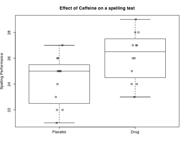
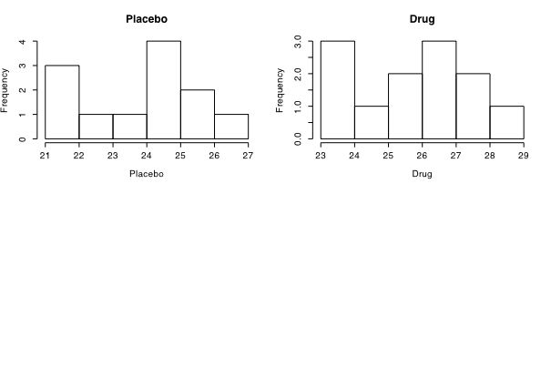
library(psych) #make sure the psych package is installed and loaded
#now, copy the data into the clipboard and then read it into R
experiment.1 <- read.clipboard()   

experiment.1    #show the data, to make sure we got it

summary(experiment.1)   #basic descriptive statistics
describe(experiment.1)  #another way to get descriptive statistics
#now some simple descriptive graphics
#The boxplot shows the Tukey 5 numbers
boxplot(experiment.1,main="Effect of Caffeine on a spelling test",ylab="Spelling Performance")  
#a stripchart shows the actual data points
stripchart(experiment.1,method="jitter",jitter=.05,vertical=T,add=T) 
#show the raw data as well added to the boxplot

multi.hist(experiment.1) #show the histograms if we want
with(experiment.1, t.test(Placebo,Drug,equal.var=TRUE) )   #the t-test 

The code above produces this output:

> experiment.1    #show the data, to make sure we got it
   Placebo Drug
1       24   24
2       25   29
3       27   26
4       26   23
5       26   25
6       22   28
7       21   27
8       22   24
9       23   27
10      25   28
11      25   27
12      25   26
> 
> summary(experiment.1)   #basic descriptive statistics
    Placebo           Drug      
 Min.   :21.00   Min.   :23.00  
 1st Qu.:22.75   1st Qu.:24.75  
 Median :25.00   Median :26.50  
 Mean   :24.25   Mean   :26.17  
 3rd Qu.:25.25   3rd Qu.:27.25  
 Max.   :27.00   Max.   :29.00  
> describe(experiment.1)  #another way to get descriptive statistics
        var  n  mean   sd median trimmed  mad min max range  skew kurtosis   se
Placebo   1 12 24.25 1.86   25.0    24.3 1.48  21  27     6 -0.33    -1.33 0.54
Drug      2 12 26.17 1.85   26.5    26.2 2.22  23  29     6 -0.22    -1.33 0.53
> #now some simple descriptive graphics
> boxplot(experiment.1,main="Effect of Caffeine on a spelling test",ylab="Spelling Performance")   #show some basic descriptive graphics
> stripchart(experiment.1,method="jitter",jitter=.05,vertical=T,add=T)  #show the raw data as well added to the boxplot
> 
> multi.hist(experiment.1) #show the histograms if we want

The t-test (equal sample sizes)

> with(experiment.1, t.test(Placebo,Drug,equal.var=TRUE) )   #the t-test 

	Welch Two Sample t-test

data:  Placebo and Drug 
t = -2.5273, df = 21.999, p-value = 0.01918
alternative hypothesis: true difference in means is not equal to 0 
95 percent confidence interval:
 -3.4894368 -0.3438965 
sample estimates:
mean of x mean of y 
 24.25000  26.16667 

t-test, unequal sample sizes -- two ways

Missing values are specified by NA

Missing values are specified by NA

   Placebo Drug
1       24   24
2       25   29
3       27   26
4       26   23
5       26   25
6       22   28
7       21   27
8       22   24
9       23   27
10      25   28
11      25   27
12      25   26
13      22   NA
14      25   NA

#copy the data into the clipboard, read the clipboard, and then do the normal t-test.
 
exp.1 <- read.clipboard()  #make sure the data are in the clipboard
with(exp.1, t.test(Placebo,Drug,equal.var=TRUE) )

Produces this output:

> exp.1 <- read.clipboard()
> with(exp.1, t.test(Placebo,Drug,equal.var=TRUE) )

	Welch Two Sample t-test

data:  Placebo and Drug 
t = -2.7917, df = 23.327, p-value = 0.01028
alternative hypothesis: true difference in means is not equal to 0 
95 percent confidence interval:
 -3.5223056 -0.5253134 
sample estimates:
mean of x mean of y 
 24.14286  26.16667 

or, if the data are strung out

   spelling conditions
1      24    Placebo
2      25    Placebo
3      27    Placebo
4      26    Placebo
5      26    Placebo
6      22    Placebo
7      21    Placebo
8      22    Placebo
9      23    Placebo
10     25    Placebo
11     25    Placebo
12     25    Placebo
13     22    Placebo
14     25    Placebo
15     24       Drug
16     29       Drug
17     26       Drug
18     23       Drug
19     25       Drug
20     28       Drug
21     27       Drug
22     24       Drug
23     27       Drug
24     28       Drug
25     27       Drug
26     26       Drug

 
exp.3 <- read.clipboard()
with(exp.3, t.test(spelling~conditions)

> exp.3 <- read.clipboard()
> with(exp.3,t.test(spelling~conditions))

	Welch Two Sample t-test

data:  spelling by conditions 
t = 2.7917, df = 23.327, p-value = 0.01028
alternative hypothesis: true difference in means is not equal to 0 
95 percent confidence interval:
 0.5253134 3.5223056 
sample estimates:
   mean in group Drug mean in group Placebo 
             26.16667              24.14286