This is a very brief guide to help students in a research methods course make use of the R statistical language to analyze some of the data they have collected. For more extensive tutorials of R in psychology, see my short and somewhat longer tutorials as well as the much more developed tutorial by Jonathan Baron and Yuelin Li. (Note that the blue text may be directly copied into R)
However, to do analyses on your own machine, you will need to download the R program from the R project and install it yourself. Go to the R home page and then choose the Download from CRAN (Comprehensive R Archive Network) option. This will take you to list of mirror sites around the world. The most convenient mirror is simply the cloud. You may download the Windows, Linux, or Mac versions at this site. Installation differs across platforms but, at least for a Mac, is very easy.
Run R with a text editor to save your commands for later use. Or, use the edit window in R to write out your commands as you work. Save this file for later use.
R is case sensitive and does not give overly useful diagnostic messages. If you get an error message, don't be flustered but rather be patient and try the command again using the correct spelling for the command.
When in doubt, use the help () function. This is identical to the ? function where function is what you want to know about. e.g.,
? read.table    #ask for help in using the read.table function  -- see the answer in its own window
#or
help (read.table) #another way of asking for help.  - see the window
The psych package may be downloaded from CRAN either by using the package installer menu option or by directly installing it:
install.packages("psych", dependencies=TRUE)
install.packages)("psychTools")
For most data analysis, rather than manually enter the data into R, it is probably more convenient to use a spreadsheet (e.g., Excel or OpenOffice) as a data editor, save as a tab or comma delimited file, and then read the data from that file or read from the clipboard using the read.clipboard() command. (found in the psych package).
For analysing the data from the computer simulation, the data are already in a readable form, with labels for the variables in the first row. If you have run multiple experiments, there are some comment lines that need to be removed before reading into R. Most of the examples in this tutorial assume that the data have been entered this way. Many of the examples in the help menus have small data sets entered using the c() command or created on the fly.
For the example, we read data from the local computer for 100 cases of simulated data with 5 independent variables and 3 dependent variables. In addition, the simulation has already done some recoding, converting two of the independent variables into 2 (IMP_2) or 3 (TOD_3) categories.
To read a file from your local machine, change the datafilename to specify the path to the data. A simple trick on the Mac is to store the datafile on your desktop. Thus the path is "Desktop/myfilename".
If you have opened the file using a text editor or Excel, you can just copy the appropriate rows into the clipboard and then use the "read.clipboard()" command.
#If I want to read a datafile from my desktop
datafilename <- "Desktop/205 Simulations Stuff/Simulation.Data"

#now read the data file
sim.data  <- read.table(datafilename,header=TRUE)  #read the data file

#Alternatively, to read in a comma delimited file:
#my.data  <- read.table(datafilename,header=TRUE,sep=",")

#alternatively, copy the data into the clipboard and
sim.data <- read.clipboard()


names(sim.data)  #list the names of the variables
attach(sim.data)  #makes the variables available for later analysis


#results in this output

> datafilename <- "Desktop/Simulation.Data"
> sim.data  <- read.table(datafilename,header=TRUE)  #read the data file
> names(sim.data)  #list the names of the variables
 [1] "trials"      "drug"        "time"        "anxiety"     "impulsivity" "sex"         "arousal"     "tension"
 [9] "performance" "IMP_2"       "TOD_3"
> attach(sim.data)  #makes the variables available for later analysis

V dim(sim.data)     #how many variables and how many subjects?
[1] 100  11
If you first make the psych package active, then we can describe the data:
library(psych)   #you only need to do this once.

describe(sim.data)
             mean    sd  skew   n median   se
trials      50.50 29.01  0.00 100   50.5 2.90
drug         0.44  0.50  0.24 100    0.0 0.05
time        15.19  4.47 -0.08 100   15.0 0.45
anxiety      5.42  1.95 -0.24 100    5.0 0.20
impulsivity  5.03  2.14  0.18 100    5.0 0.21
sex          1.46  0.50  0.16 100    1.0 0.05
arousal     64.29  7.21 -0.51 100   66.0 0.72
tension     58.68  7.16 -0.28 100   59.0 0.72
performance 80.00 12.23 -0.85 100   83.0 1.22
IMP_2        1.53  0.50 -0.12 100    2.0 0.05
TOD_3        2.12  0.77 -0.20 100    2.0 0.08


alternatively, we can simply summarize them using the summary command.  I do not find this as useful as describe.

summary(sim.data)
     trials            drug           time          anxiety       impulsivity         sex          arousal         tension
 Min.   :  1.00   Min.   :0.00   Min.   : 8.00   Min.   : 0.00   Min.   : 0.00   Min.   :1.00   Min.   :48.00   Min.   :40.00
 1st Qu.: 25.75   1st Qu.:0.00   1st Qu.:12.00   1st Qu.: 4.00   1st Qu.: 4.00   1st Qu.:1.00   1st Qu.:58.75   1st Qu.:54.00
 Median : 50.50   Median :0.00   Median :15.00   Median : 5.00   Median : 5.00   Median :1.00   Median :66.00   Median :59.00
 Mean   : 50.50   Mean   :0.44   Mean   :15.19   Mean   : 5.42   Mean   : 5.03   Mean   :1.46   Mean   :64.29   Mean   :58.68
 3rd Qu.: 75.25   3rd Qu.:1.00   3rd Qu.:19.00   3rd Qu.: 7.00   3rd Qu.: 7.00   3rd Qu.:2.00   3rd Qu.:70.00   3rd Qu.:63.00
 Max.   :100.00   Max.   :1.00   Max.   :22.00   Max.   :10.00   Max.   :10.00   Max.   :2.00   Max.   :75.00   Max.   :74.00
  performance      IMP_2          TOD_3
 Min.   : 45   Min.   :1.00   Min.   :1.00
 1st Qu.: 73   1st Qu.:1.00   1st Qu.:2.00
 Median : 83   Median :2.00   Median :2.00
 Mean   : 80   Mean   :1.53   Mean   :2.12
 3rd Qu.: 88   3rd Qu.:2.00   3rd Qu.:3.00
 Max.   :100   Max.   :2.00   Max.   :3.00


> summary(sim.data[,2:5])    #summarize a subset
      drug           time          anxiety       impulsivity
 Min.   :0.00   Min.   : 8.00   Min.   : 0.00   Min.   : 0.00
 1st Qu.:0.00   1st Qu.:12.00   1st Qu.: 4.00   1st Qu.: 4.00
 Median :0.00   Median :15.00   Median : 5.00   Median : 5.00
 Mean   :0.44   Mean   :15.19   Mean   : 5.42   Mean   : 5.03
 3rd Qu.:1.00   3rd Qu.:19.00   3rd Qu.: 7.00   3rd Qu.: 7.00
 Max.   :1.00   Max.   :22.00   Max.   :10.00   Max.   :10.00
>
To find the correlation between a set of variables, use the cor command:
round(cor(sim.data),2)    #round the correlations to 2 decimals


            trials  drug  time anxiety impulsivity   sex arousal tension performance IMP_2 TOD_3
trials        1.00  0.00 -0.05    0.06       -0.03 -0.05   -0.01   -0.33        0.06  0.06 -0.06
drug          0.00  1.00  0.14   -0.04        0.18 -0.05    0.49    0.42        0.38  0.07  0.20
time         -0.05  0.14  1.00    0.15        0.04 -0.12    0.78    0.14        0.70  0.00  0.94
anxiety       0.06 -0.04  0.15    1.00        0.06 -0.12    0.19    0.42        0.20 -0.02  0.13
impulsivity  -0.03  0.18  0.04    0.06        1.00 -0.13    0.03    0.05        0.03  0.82  0.02
sex          -0.05 -0.05 -0.12   -0.12       -0.13  1.00   -0.24   -0.07       -0.24 -0.14 -0.09
arousal      -0.01  0.49  0.78    0.19        0.03 -0.24    1.00    0.24        0.87  0.00  0.80
tension      -0.33  0.42  0.14    0.42        0.05 -0.07    0.24    1.00        0.19 -0.10  0.18
performance   0.06  0.38  0.70    0.20        0.03 -0.24    0.87    0.19        1.00  0.00  0.70
IMP_2         0.06  0.07  0.00   -0.02        0.82 -0.14    0.00   -0.10        0.00  1.00 -0.01
TOD_3        -0.06  0.20  0.94    0.13        0.02 -0.09    0.80    0.18        0.70 -0.01  1.00
However, to make neater output, you could use the LowerCor function. To find the correlation between a set of variables, use the cor command:
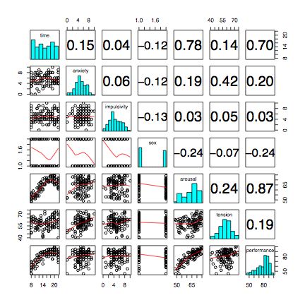
For a limited number of variables, we can also show scatter plot matrices of all the relationships.
pairs.panels(sim.data) #shows the scatter plots and correlations of all the variables

To show the relationship between any two variables use plot.
plot(impulsivity,performance)

Graphical output goes to a graphics window. This may be saved as a pdf using the save command (in the menus) and then printed in another document. On a mac, a new graphics window may be created by the quartz(height=6, width=6) command (height and width specified for nice looking output on a printer.)
quartz(height=6, width=6)
The relationship between variables is seen graphically in the plot command (see above). It is quantified with the Pearson Correlation. In case of missing values, it is necesary to specify that you want to use complete cases or pairwise deleted cases. Without rounding, the output is to 5 decimals. Rounding to 2 decimals is most appropriate.
For analysis of variance of categorical variables, we can use the aov() function:
aov.1 <- aov(arousal ~ drug,data=sim.data) #one way ANOVA of drug
summary(aov.1) #summary table
print(model.tables(aov.1,"means"),digits=3) #the means
aov.2 <- aov(arousal ~ TOD_3,data=sim.data) #one way ANOVA of time of day
summary(aov.2) #summary table
print(model.tables(aov.2,"means"),digits=3) #the means
aov.3 <- aov(arousal ~ drug * TOD_3,data=sim.data) # 2 way ANOVA
summary(aov.3)
print(model.tables(aov.3,"means"),digits=3)
which produces this output:
aov.1 <- aov(arousal ~ drug ,data=sim.data)
print(model.tables(aov.1,"means"),digits=3)
Tables of means
Grand mean
64.29
drug
drug
0 1
61.2 68.3
TOD_3
TOD_3
1 2 3
57.0 63.5 70.0
drug:TOD_3
TOD_3
drug 1 2 3
0 54.5 61.3 68.0
1 59.4 66.3 73.1
> summary(aov.1)
Df Sum Sq Mean Sq F value Pr(>F)
drug 1 1246.31 1246.31 91.5979 1.244e-15 ***
TOD_3 1 2594.00 2594.00 190.6467 < 2.2e-16 ***
drug:TOD_3 1 0.08 0.08 0.0058 0.9397
Residuals 96 1306.21 13.61
---
Signif. codes: 0 �***� 0.001 �**� 0.01 �*� 0.05 �.� 0.1 � � 1
>
To produce graphs from this analysis, we can use the plot and lines commands. We will do 2 graphs, one of the effect of Time of Day on arousal, the other of the (non-significant) interaction of the drug by time of day.
tod <- c(8,15,22)   #the values of the X axis
arouse <- c(57.0, 63.5, 70.0)  #copy the results from the means output
plot(tod,arouse,type="b", ylab="arousal",xlab="time of day",ylim=c(0,100))

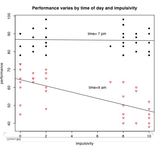
The next set of instructions allow us to consider the interaction of categorical variables with continuous variables. The data are from a simulation of performance varying by time of day and impulsivity. (Note, for the analysis of the 205 simulation, you need to make sure you use your data, not the example data set used here.)
One can graph the data points and the regression lines (which I show), or just the regression lines.
datafilename="http://personality-project.org/r/datasets/simulations.txt"  #web copy of data file
sim.data =read.table(datafilename,header=TRUE)  #read the data file
attach(sim.data)     #make the sim.data the active set

#the next commands allow for a more generic set of plotting commands
#rather than replace the variabless DV, IV1, and IV2, just enter their names in models.

DV=performance   #The Dependent Variable
IV1=impulsivity  #continuous Independent Variable
IV2=time        #categorical Independent Variable

mydata=data.frame(DV,IV1,IV2)   #put them together into one data frame
attach(mydata)

zmydata=data.frame(scale(mydata))             #convert the data to standard scores to do the regression analysis
                                              #this makes the interaction term independent of the main effects
model=lm(DV~IV1+IV2+ IV1*IV2,data=zmydata)    #test the main effects of IV1 and IV2 and the interaction of IV1 and IV2
print(model)              #just show the coefficients
summary(model)            #show the coefficients as well as the probability estimates for the coefficients


by(mydata,IV2,function(x) summary(lm(DV~IV1,data=x))) #give the summary stats for the regression DV~IV1 for each value of IV2

par(mfrow=c(1,1))                      #set the graphics back to a 1 x 1 plot
symb=c(19,25,3,23)                     #choose some nice plotting symbols
colors=c("black","red","green","blue") #choose some nice colors

cat.iv=as.integer(IV2 < 10) +1       #convert IV2 to a categorical variable with 2 values of 1 and 2

                              #now draw the DV~IV1 regression for each value of IV2
plot(IV1,DV,pch=symb[cat.iv],col=colors[cat.iv],cex=1.0,xlab="label for x axis",ylab="label for y axis",main="overall label goes here")   #show  the data points
by(mydata,IV2,function(x) abline(lm(DV~IV1,data=x)))  #show the best fitting regression for each group

text(6,60,"label for cat.iv=1")      #adjust the x, y coordinates to fit the graph
text(6,90,"label for cat.iv =2 ")

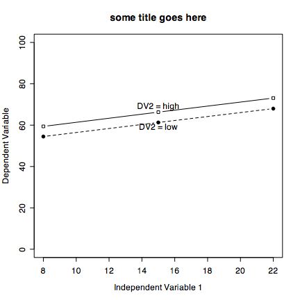
It is also easy to draw plots of specific points connected by lines. Consider if we have the experimental results on a Dependent Variable (DV) as a function of two Independent Variables (IV1 and IV2). Specifically, consider the results from aov.3 (above). Although in this example I refer to them generically, obviously one should change the labels to fit the data.)
| IV 1 (time of day) | |||
| Low | Medium | High | |
| IV 2 Low (Placebo) | 54.5 | 61.3 | 68.0 |
| IV 2 High (Caffeine | 59.4 | 66.3 | 73.1 |
These results can be drawn using plot and lines. Create a variable IV1 for the values on the X axis. Then create two sets of coordinates of the DV, one for each level of the IV2. Then, use plot and lines.
quartz(height=6,width=6)   #create a new graphics window for this plot (mac)
IV1 <- c(8,15,22)    #the values of the first Independent Variable (time of day)

iv2low=c(54.5, 61.3 ,68.0)  #the Dependent variable values for low, medium and high IV 1 and low IV2
iv2high=c(59.4, 66.3, 73.1) #the Dependent variable values for low, mediuam and high IV 1 and high IV2
IV1 <- c(8,15,22)    #the values of the first Independent Variable

plot(IV1,iv2low,xlim=c(8,22),ylim=c(0,100),type="b",lty="dashed", xlab="Independent Variable 1" ,ylab="Dependent Variable",  pch=19,main="some title goes here")    #plot character is closed circle

lines(IV1,iv2high,,pch=22,type="b") #plot character is an open square
text(15,60,"DV2 = low")    #change the location of these labels to fit the data
text(15,70,"DV2 = high")

Suppose we have a three way interaction and want to make a two panel graph. Then we specify that we want a graphic with 2 columns and 1 row, and then draw the graphics twice.
par(mfrow=c(1,2))    #a 1 row, 2 column graph

IV1 <- c(8,15,22)    #the values of the first Independent Variable (time of day)

iv2low=c(54.5, 61.3 ,68.0)  #the Dependent variable values for low, medium and high IV 1 and low IV2
iv2high=c(59.4, 66.3, 73.1) #the Dependent variable values for low, mediuam and high IV 1 and high IV2
IV1 <- c(8,15,22)    #the values of the first Independent Variable

plot(IV1,iv2low,xlim=c(8,22),ylim=c(0,100),type="b",lty="dashed", xlab="Independent Variable 1" ,ylab="Dependent Variable",  pch=19,main="some title goes here")    #plot character is closed circle

lines(IV1,iv2high,,pch=22,type="b") #plot character is an open square
text(15,60,"DV2 = low")    #change the location of these labels to fit the data
text(15,70,"DV2 = high")

#now do the second figure (aribitray numbers)

IV1 <- c(8,15,22)    #the values of the first Independent Variable (time of day)

iv2low=c(44.5, 71.3 ,68.0)  #the Dependent variable values for low, medium and high IV 1 and low IV2
iv2high=c(69.4, 66.3, 53.1) #the Dependent variable values for low, mediuam and high IV 1 and high IV2
IV1 <- c(8,15,22)    #the values of the first Independent Variable

plot(IV1,iv2low,xlim=c(8,22),ylim=c(0,100),type="b",lty="dashed", xlab="Independent Variable 1" ,ylab="Dependent Variable",  pch=19,main="another title goes here")    #plot character is closed circle

lines(IV1,iv2high,,pch=22,type="b") #plot character is an open square
text(15,40,"DV2 = low")    #change the location of these labels to fit the data
text(15,80,"DV2 = high")

More extensive discussions of the use of R in psychology may be found in my short and somewhat longer tutorials as well as the much more developed tutorial by Jonathan Baron and Yuelin Li. Finally, when in doubt, it doesn't hurt to consult the help pages or do a "help.search("some string") command.