Testing Circumplex Structure

A number of elementary requirements can be teased out of the idea of circumplex structure. First, circumplex structure implies minimally that variables are interrelated; random noise does not a circumplex make. Second, circumplex structure implies that the domain in question is optimally represented by two and only two dimensions. Third, circumplex structure implies that variables do not group or clump along the two axes, as in simple structure, but rather that there are always interstitial variables between any orthogonal pair of axes (Saucier, 1992). In the ideal case, this quality will be reflected in equal spacing of variables along the circumference of the circle (Gurtman, 1994; Wiggins, Steiger, & Gaelick, 1981). Fourth, circumplex structure implies that variables have a constant radius from the center of the circle, which implies that all variables have equal communality on the two circumplex dimensions (Fisher, 1997; Gurtman, 1994). Fifth, circumplex structure implies that all rotations are equally good representations of the domain (Conte & Plutchik, 1981; Larsen & Diener, 1992)." (Acton and Revelle, 2004)

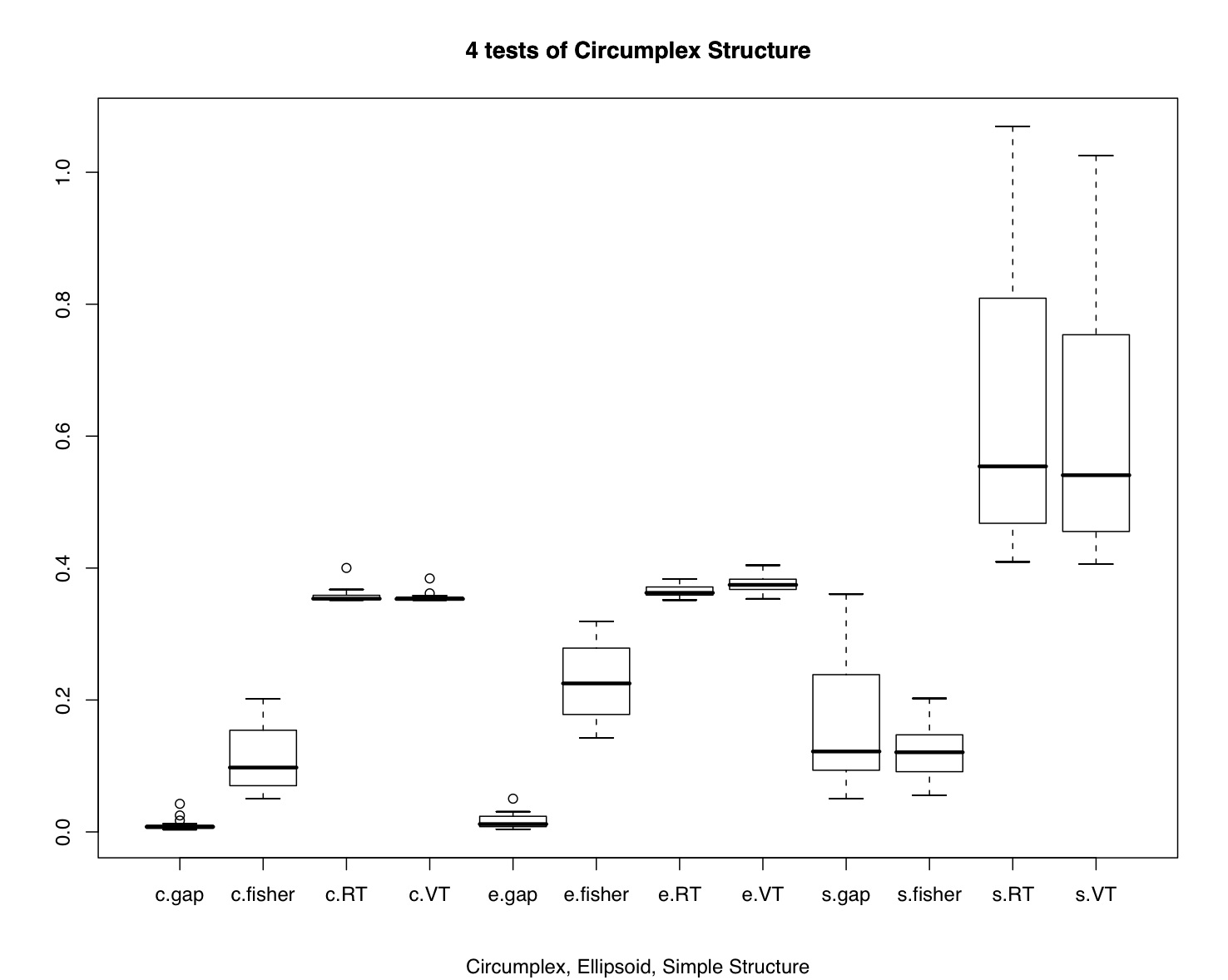
Acton and Revelle reviewed the effectiveness of 10 tests of circumplex structure and found that four did a particularly good job of discriminating circumplex structure from simple structure, or circumplexes from ellipsoidal structures. Unfortunately, their work was done in Pascal and is not easily available. Here we release R code to do the four most useful tests:

• The Gap test of equal spacing
• Fisher's test of equality of axes
• A test of indifference to Rotation
• A test of equal Variance of squared factor loadings across arbitrary rotations.

Included in this set of functions is simple procedure to generate circumplex structured or simple structured data, the four test statistics, and a simple simulation showing the effectiveness of the four procedures. All of these functions are part of the psych package available at CRAN.

Generating circumplex data

This function generates simple structured or circumplex data. This is adapted from code developed for the Rafaeli and Revelle analysis of mood data.

circ.sim <- function (nvar = 72 ,nsub = 500, 
    circum = TRUE, xloading =.6, yloading = .6, gloading=0, xbias=0,  ybias = 0,categorical=FALSE, low=-3,high=3,truncate=FALSE,cutpoint=0) 
	{ 
	avloading <- (xloading+yloading)/2
	
	errorweight <- sqrt(1-(avloading^2  + gloading^2))  #squared errors and true score weights add to 1
    g <- rnorm(nsub) 
	truex <- rnorm(nsub)* xloading  +xbias #generate normal true scores for x + xbias
	truey <- rnorm(nsub) * yloading + ybias #generate normal true scores for y + ybias

	if (circum)  #make a vector of radians (the whole way around the circle) if circumplex
	{radia <- seq(0,2*pi,len=nvar+1)  
      rad <- radia[which(radia<2*pi)]        #get rid of the last one
     } else rad <- rep(seq(0,3*pi/2,len=4),nvar/4) #simple structure 
        
	error<- matrix(rnorm(nsub*(nvar)),nsub)    #create normal error scores

	#true score matrix for each item reflects structure in radians
	trueitem <- outer(truex, cos(rad)) + outer(truey,sin(rad)) 

	item<- gloading * g +  trueitem  + errorweight*error   #observed item = true score + error score 
    if (categorical) {
        
    	item = round(item)       #round all items to nearest integer value
		item[(item<= low)] <- low     
		item[(item>high) ] <- high   
		}
	if (truncate) {item[item < cutpoint] <- 0  }
	return (item) 
	}  

Circumplex Tests

This function (including four embedded functions to do the separate tests) applies four tests of circumplex fit. These functions make use of the factor.rotate function from the psych package, but I include that function here for ease of use.

factor.rotate <-
function(f,angle,col1,col2)  {
   #hand rotate two factors from a loading matrix
   #see the GPArotation package for much more elegant procedures
     nvar<- dim(f)[2]
     rot<- matrix(rep(0,nvar*nvar),ncol=nvar)
     rot[cbind(1:nvar, 1:nvar)] <- 1
     theta<- 2*pi*angle/360
     rot[col1,col1]<-cos(theta)
     rot[col2,col2]<-cos(theta)
     rot[col1,col2]<- -sin(theta)
     rot[col2,col1]<- sin(theta)
     result <- f %*% rot
     return(result) }
circ.tests <- function(loads,loading=TRUE,sorting=TRUE) {

circ.gap <- function(loads,loading=TRUE,sorting=TRUE) {
if (loading) {l <- loads$loadings} else { 
       l <- loads}
       l<- l[,1:2]
    commun=rowSums(l*l) 
    theta=sign(l[,2])*acos(l[,1]/sqrt(commun)) #vector angle in radians
    if(sorting) {theta<- sort(theta)}
    gaps <- diff(theta)
    test <- var(gaps)
    return(test)
    }


circ.fisher <- function(loads,loading=TRUE) {
if (loading) {l <- loads$loadings} else { 
       l <- loads}
       l<- l[,1:2]
   radius <- rowSums(l * l)
   test <- sd(radius)/mean(radius)
  return (test)
  }
  
  
  circ.rt <- function(loads,loading=TRUE) {
 if (loading) {l <- loads$loadings} else { 
       l <- loads}
       l<- l[,1:2]
       qmc <- rep(0,10)
       for (i in 0:9) {theta <- 5*i
       	rl <- factor.rotate(l,theta,1,2)
       	 l2 <- rl*rl
       qmc[i] <- sum(apply(l2,1,var)) }
       test <- sd(qmc)/mean(qmc)
 }
 
 circ.v2 <- function(loads,loading=TRUE) {
if (loading) {l <- loads$loadings} else { 
       l <- loads}
       l<- l[,1:2]
   crit <- rep(0,10)
       for (i in 0:9) {
       		theta <- 5*i
       		rl <- factor.rotate(l,theta,1,2)
       	 	l2 <- rl*rl
       	 	suml2 <- sum(l2)
       		crit[i] <- var(l2[,1]/suml2)
       }
       test <- sd(crit)/mean(crit)
  return (test)
  }
 

   gap.test <- circ.gap(loads,loading,sorting)
   fisher.test <- circ.fisher(loads,loading)
   rotation.test <- circ.rt(loads,loading)
   variance.test <- circ.v2(loads,loading)
   circ.tests <- list(gaps=gap.test,fisher=fisher.test,RT=rotation.test,VT=variance.test)
   }
   
   

Demonstrating the tests

This final function simulates 16 different data sets.

circ.simulation <- function()
 {samplesize <- c(100,200,400,800)
  numberofvariables <- c(16,32,48,72)
  results <- matrix(NA,ncol=4,nrow=16)
  results.ls <- list()
   case <- 1
  for (ss in 1:4) {
    for (nv in 1:4) {
    
      circ.data <- circ.sim(nvar=numberofvariables[nv],nsub=samplesize[ss])
      sim.data <-  circ.sim(nvar=numberofvariables[nv],nsub=samplesize[ss],circum=FALSE)
      elipse.data <- circ.sim(nvar=numberofvariables[nv],nsub=samplesize[ss],yloading=.4)
      r.circ<- cor(circ.data)
      r.sim <- cor(sim.data)
      r.elipse <- cor(elipse.data)
      pc.circ <- principal(r.circ,2)
      pc.sim <- principal(r.sim,2)
      pc.elipse <- principal(r.elipse,2)
      case <- case + 1
      results.ls[[case]] <- list(numberofvariables[nv],samplesize[ss],circ.tests(pc.circ),circ.tests(pc.elipse),circ.tests(pc.sim))
     }
     }
     results.mat <- matrix(unlist(results.ls),ncol=14,byrow=TRUE)
    colnames(results.mat) <- c("nvar","n","c-gap","c-fisher","c-RT","c-VT","e-gap","e-fisher","e-RT","e-VT","s-gap","s-fisher","s-RT","s-VT")
    results.df <- data.frame(results.mat)
 	 return(results.df)
  }
  
 
 demo <- circ.simulation()
 boxplot(demo[3:14])
 title("4 tests of Circumplex Structure",sub="Circumplex, Ellipsoid, Simple Structure")