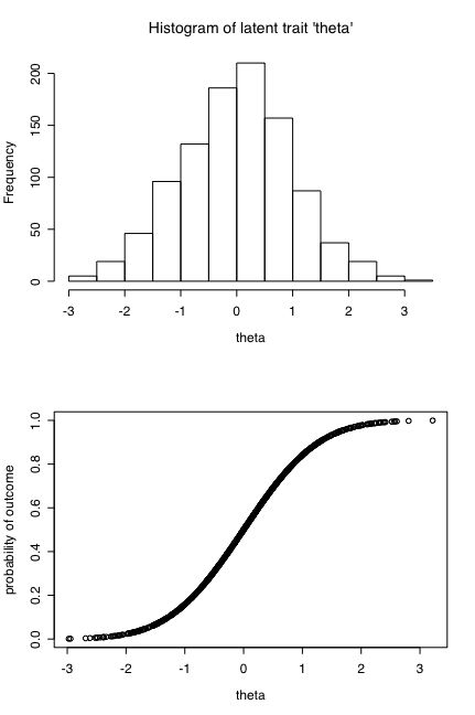
Figure 1: Hypothetical relationship between an underlying trait (theta) and the probability of an action/outcome. Theta is distributed normally, the probability function is the cumulative normal.
I address two questions: 1) Is a correlation of .3 surprising? and 2) is such a correlation useful for understanding or predicting real world criteria?
The answer to the first question is no, it is not surprising, but merely what one would expect given most of our outcome measures are dichotomous (success/failure, act or withhold action) and that underlying latent traits do not predict outcomes, but rather the probability of an outcome.
Consider the following scenario: There is a latent trait (theta) that is normally distributed in the population. Surface (observed) manifestations of this trait (X1 ... Xn) are probalistic with the probability increasing as a function of theta. Assume that the probability function is the cumulative normal, that is, for values of theta at the mean of theta, the probability of Xi = .5. For values of theta that are one standard deviation below the mean, p(Xi = .16). For values of theta one standard deviations above the mean, p(Xi) = .84). These two assumptions are shown in Figure 1:
Figure 1: Hypothetical relationship between an underlying trait (theta) and the probability of an action/outcome. Theta is distributed normally, the probability function is the cumulative normal.
Given the latent trait, theta, we can simulate the pattern of responses to items X1 ... Xn for subjects 1 ... N by assigning for each item a value of 0 or 1 with a probability of a 1 defined as the cumulative normal value of theta (see Figure 1 b). (The computer code for these simulations is shown as an Appendix.) This means that someone at a value of 1 theta is 1.69 times as likely to endorse an item (get a 1) than is someone with theta of 0 and 5.3 times as likely to endorse an item than is someone with a value of -1 theta.
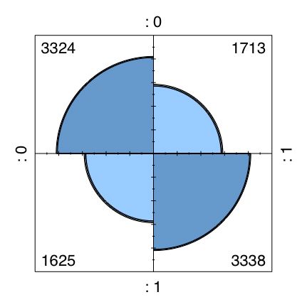
Although these differences in probabilities seem very large and lead to the intuition that any two such items should be highly correlated, in fact they produce two by two tables similar to the following:
| Item 1 | |||
| 0 | 1 | ||
| Item 2 | |||
| 0 | 17% | 33% | |
| 1 | 33% | 17% |
The correlation of an item with the "true score" or theta dimension is a point-biserial correlation of approximately .57. The results are similar to the following analyses (shown for both the theta dimension as well as the probability dimension).
| Item 1 | |||
| 0 | 1 | ||
| Theta | -.57 | .57 | |
| Prob | .33 | .67 |
As is well known, scales made up by combining correlated items are much more reliable than individual items. Since scale validity is bounded by the square root of the scale reliability, we would expect the correlation with true score of a scale made up of items X1 ... Xn to increase as we add more items. This is indeed the case. Although a single item correlates .57 with the true score, as we increase from the number of items from 1 to 32, the reliability of pooled scale increases from .33 to .94 and the corresponding correlation with the "true score" increases from .57 to .97.
| Number of items | alpha | r with true |
| 1 | .33 | .57 |
| 2 | .48 | .70 |
| 4 | .67 | .82 |
| 8 | .80 | .89 |
| 16 | .89 | .94 |
| 32 | .94 | .97 |
Although the underlying, latent distribution in all of these simulations is normal, it is interesting to note that the distribution of the aggregated scores approaches a rectangular distribution. That is, we can not make inferences about the underlying latent variable distribution from the observed distribution.
Although it is true that less than 10% of the variance in item X2 is accounted for by knowing the value of item X1, it is also the case that having a high score on item X1 leads to a high score on item X21 twice as often as does a low score. Such an odds ratio of 2 (.34/.17) is terribly useful if the cost of failure (a 0 on item 2) is high or the benefits of success (a 1 on item 2) is high.
The results discussed above were generated using the R statistical package and the following very simple code (For a tutorial on the use of R):
#Simulations to represent personality correlations
#first define a function to find coefficient alpha
alpha.scale=function (x,y) #create a reusable function to find coefficient alpha
#input to the function are a scale and a data.frame of the items in the scale
{
Vi=sum(diag(var(y,na.rm=TRUE))) #sum of item variance
Vt=var(x,na.rm=TRUE) #total test variance
n=dim(y)[2] #how many items are in the scale? Calculated dynamically
((Vt-Vi)/Vt)*(n/(n-1))} #alpha
#define basic parameters
numberofcases=10000 #specify the number of subjects
numberofvariables=8 #and the number of variables
low= 0 #easist item
high=0 #hardest item
difficulty =seq(low, high, length=numberofvariables) #spread the items out
distro=rnorm(numberofcases,0,1) #make up a normal distribution
true=pnorm(distro) #trait scores are cumulative normals
error <- matrix(runif(numberofcases*numberofvariables),nrow=numberofcases,ncol=numberofvariables) #matrix of uniform random numbers
observed <- matrix(rep(0,numberofcases*numberofvariables),nrow=numberofcases,ncol=numberofvariables) #set all scores to 0
observed[error<(true-difficulty)]<-1 #if the random number (error) is less than the true score, then the item is "correct"
pooled=rowSums(observed)/dim(observed)[2] #total across all items (expressed in 0-1 metric)
print("alpha reliability = ")
round(alpha.scale(pooled*numberofvariables,observed),2) #find alpha but correct of 0-1 metric
combined.df=data.frame(distro,true,observed,pooled) #make up a summary data frame
cors=cor(combined.df) #find the correlations
round(cors,2) #print the rounded correlations
#quartz(width=6,height=9) #make a graphics window
par(mfrow=c(4,1)) #number of rows and columns to graph
hist(distro,xlab="theta",main="Histogram of latent trait 'theta'",freq=FALSE)
plot(distro,true,xlab="theta",ylab="probability of outcome")
hist(pooled,freq=FALSE)
plot (distro,pooled,xlab="theta",ylab="average score")
t12=table(combined.df$X1,combined.df$X2)
fourfoldplot(t12) #a cute way of showing a two by two table
t.test(distro~X1,data=combined.df)
t.test(true~X1,data=combined.df)
low=subset(combined.df,X1==0) #form two subsets and then plot them
high=subset(combined.df,X1>0)
hl=hist(low$distro,density=5,plot=FALSE) #find but do not show histogram stats
hh=hist(high$distro,plot=FALSE,density=5,angle=135)
#plot them both as overlapping distributions
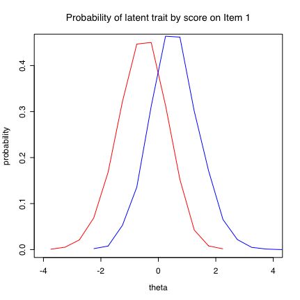
plot(hl$mids,hl$density,xlim=c(-4,4),type="l",col="red",xlab="theta",ylab="probability",main="Probability of latent trait by score on Item 1")
lines(hh$mids,hh$density,type="l",col="blue")