In order to analyse the effect of bipolar vs. unipolar scales in the measurement of emotion we generated multiple sets of artificial data with known structure. Structural analyses of these data sets were done using exploratory factor analysis and the Very Simple Structure criterion (Revelle and Rocklin, 1979) to determine the most interpretable number of factors.
These analyses were all done using the public domain statistical and data handling computer system R (R Development Core Team, 2004). To facilitate others who want to replicate or extend our analyses, we include in this appendix the original R code for all analyses reported. The code in this appendix may be copied directly into R and executed. Very Simple Structure (Revelle and Rocklin, 1979) has been adapted for R and is available at http://personality-project.org/r/vss.html and is included in the R-package "psych" available in a repository at http://personality-project.org/r/. For a brief tutorial on the use of R in psychological research, we recommend http://personality-project.org/r
Sample sizes were chosen to represent typical sample sizes in the literature, as well as the very large sample we report in the text. Thus sample sizes of 200, 800 and 3,200 were examined. Each simulation was conducted twice, once with bipolar items (generated as described above) and once with unipolar items. Following Russell and Carroll's (1999) assumption of how unipolar items are formed, we collapsed all item scores < 0 to zero. This creates a certain level of skew for each item.
One purpose of this simulation was to show that the factor structure of items, though greatly affected by differences or non-uniformity in item skew, can be recovered using factor analysis. To further increase skew for some items, we subtracted a constant (1.0) from True score T2 before adding error and before truncation. This led to greater skew for items with positive T2 scores, and less skew for items with negative T2 scores. Because each simulated item was a mixture of T1 and T2, the greater the positive loading on T2, the greater the skew, and the greater the negative loading on T2, the smaller the skew.
Because some of the analyses we report on either the simulated data or the real data require non-typical procedures (e.g., converting (Cartesian) factor loadings into polar coordinates), we also provide the R code for these analyses.
The following R commands define three functions (simulate.items, categorical.items, and truncate.item to create artificial items with a circumplex structure and the properties of real items used to measure mood and affect.
Functions in R may be defined with default parameter values that may be varied when called. In the following code, the parameters that may be specified are:
    nvar:    the number of items to be created
    nsub:    the number of artificial subjects to be created
    circum:  a boolean variable, TRUE of circumplex structure, FALSE for simple structure.
    avloading: the average item reliability (or communality)
    xbias:  the amount of offset from 0 for the first factor
    ybias: the amount of offset from 0 for the second factor
The primary function (simulate.items) generates items formed from two independent dimensions. The items can have either a circumplex or simple structure. True scores of items are assumed to be bivariate normal, bipolar and to lie in a two dimensional space. Default values are included in the function definition, but other values may be specified when the function is executed. The # sign indicates a comment. Text colored blue may be directly executed in R.
simulate.items <- function (nvar = 72 ,nsub = 500,
    circum = TRUE, avloading =.6,  xbias=0,  ybias = -1)
{ #begin function

trueweight <- sqrt(avloading)  #<--- true weight is sqrt(of reliability)
errorweight <- sqrt(1-trueweight*trueweight) #squared errors and true score weights add to 1

truex <- rnorm(nsub)  +xbias  #generate normal true scores for x + xbias
truey <- rnorm(nsub)  + ybias  #generate normal true scores for y + ybias

if (circum)  #make a vector of radians (the whole way around the circle) if circumplex
	{radia <- seq(0,2*pi,len=nvar+1)
	rad <- radia[which(radia<2*pi)]        #get rid of the last one
	} else rad <- rep(seq(0,3*pi/2,len=4),nvar/4)  #simple structure

error<- matrix(rnorm(nsub*(nvar)),nsub)  	#create normal error scores
#true score matrix for each item reflects structure in rad
trueitem <- outer(truex, cos(rad)) + outer(truey,sin(rad))

item<- trueweight* trueitem  + errorweight*error    #observed item = true score + error score

return (item)  }   #the value of the function is the item matrix, ready for further analysis


#
#
#############################################################################
#
# Function to convert from continous variables to discrete (-3 <-> 3 ) categorical variables


categorical.item <-function (item)
    {item = round(item)          #round all items to nearest integer value
	item[(item<=-3)] <- -3 	 #items < 3 become -3
	item[(item>3) ] <-  3      #items >3 become 3
	return(item) }             #the function returns these categorical items


##	Function to convert a bipolar scale into a unipolar scale
#(i.e., to throw away information below a cutpoint)


truncate.item <- function(item,cutpoint=0)  #truncate values less than cutpoint to zero
	{
		item[item < cutpoint] <- 0     #item values < 0 are truncated  to zero (remove to not truncate)
		return(item)
	}
In order to compare the effect of the number of subjects and the number of items, these functions are then called in a loop varying the number of subjects, the average loading, and type of structure. The output is evaluated in terms of the Very Simple Structure Criterion and chi square goodness of fit.
#
#############################################################################
#
# simulate multiple sample sizes and examine the effect of unipolar vs. bipolar categorical items


samplesize <- c(200,800,3200)       #examine the effect of three sample sizes
nvar <- 16                          #examine the effect of the number of variables
#vss.none <- list()              #results will be stored here
vss.16 <- list()
for (i in 1:3)                   #generate three data sets of varying sample size
{ items <- simulate.items(nsub=samplesize[i])
	catitem <- categorical.item(items)
 	truncitem <- truncate.item(catitem)
	#vss.none[[i]] <- list(VSS(truncitem)) #examine the VSS criterion for the unrotated solution
	vss.16[[i]] <- list(VSS(truncitem,rotate="varimax"))  #examine VSS for the Varimax rotated solution
}

nvar <- 72
#vss.none <- list()                            #results will be stored here
vss.72 <- list()
for (i in 1:3)               #generate three data sets of varying sample size
{ items <- simulate.items(nsub=samplesize[i])
	catitem <- categorical.item(items)
 	truncitem <- truncate.item(catitem)
	#vss.none[[i]] <- list(VSS(truncitem))    #examine the VSS criterion for the unrotated solution
	vss.72[[i]] <- list(VSS(truncitem,rotate="varimax"))  #examine VSS for the Varimax rotated solution
}


nvar=72                  #results will be stored here
vss.bipolar <- list()    #compare to bipolar scales

for (i in 1:3)           #generate three data sets of varying sample size
{ items <- simulate.items(nsub=samplesize[i])
	catitem <- categorical.item(items)
 	#truncitem <- truncate.item(catitem)
	#vss.none[[i]] <- list(VSS(truncitem))      #examine the VSS criterion for the unrotated solution
	vss.bipolar[[i]] <- list(VSS(catitem,rotate="varimax"))  #examine VSS for the Varimax rotated solution
}


#now generate multiple plots
#this next set generates a 3 by 3 plot of 72 bipoloar, 72 unipolar, and 16 unipolar VSS plots for Ns=200,800, 3200

plot.new()                   #set up a new plot page
par(mfrow=c(3,3))            #3 rows and 3 columns allow us to compare results
for (i in 1:3)                #for the 3 sample sizes show the VSS plots

{ x <- as.data.frame(vss.bipolar[[i]])
VSS.plot(x,paste("N= ",samplesize[i], "\n 72 bipolar variables")) }
for (i in 1:3)
{ x <- as.data.frame(vss.72[[i]])
VSS.plot(x,paste("N= ",samplesize[i], "\n 72 unipolar variables")) }
vss.72bipolar=recordPlot()            #bipolar vs. unipolar VSS
for (i in 1:3)                #for the 3 sample sizes show the VSS plots
{ x <- as.data.frame(vss.16[[i]])
VSS.plot(x,paste("N= ",samplesize[i], "\n 16 unipolar variables")) }


plot.new()                   #set up a new plot page
par(mfrow=c(3,3))            #3 rows and 3 columns allow us to compare results
for (i in 1:3)                #for the 3 sample sizes show the VSS plots

{ x <- as.data.frame(vss.16[[i]])
plotVSS(x,paste("N= ",samplesize[i], " 16 unipolar variables")) }
for (i in 1:3)
{ x <- as.data.frame(vss.72[[i]])
plotVSS(x,paste("N= ",samplesize[i], " 72 unipolar variables")) }
vss.16v72 = recordPlot()              #16 variable vs. 72 variable
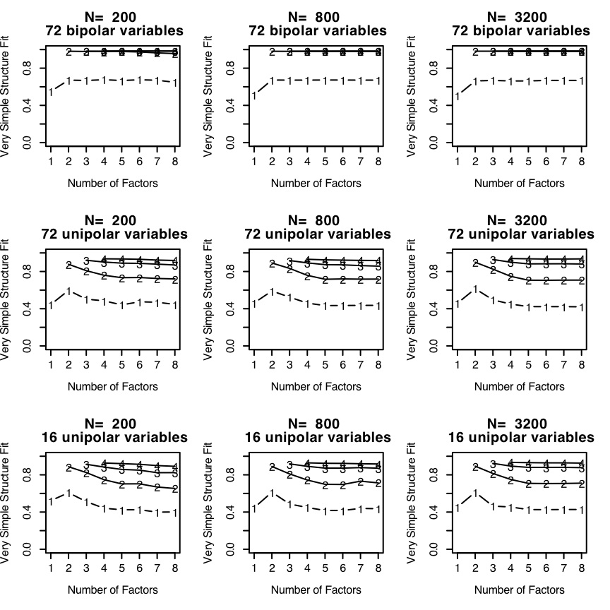
The top three panels in Figure Appendix 1 shows the Very Simple Structure criterion applied for four sample sizes (N=200,800, and 3,200) to 72 bipolar items in a circumplex structure. The middle three panels display the VSS criterion for 72 unipolar items also in a circumplex structure. The bottom three panels display the VSS criterion for 16 unipolar items.
Although it is typical to describe factor analysis results in terms of item factor loadings, it is sometimes useful to organize items in terms of polar coordinates (angles from factor 1, vector lengths as communalities), particularly when examining items in a two space. The angle function factor analyzes a data matrix, extracts two factors, rotates to a specified criterion, and then converts the loadings to polar coordinates.
angle = function(x)
{
f=factanal(x,2,"varimax")
fload=f$loadings commun=rowSums(fload*fload)
theta=sign(fload[,2])*180*acos(fload[,1]/sqrt(commun))/pi #vector angle (-180: 180)
angle <-  data.frame(x=fload[,1],y=fload[,2],communality= commun,angle=theta) return(angle) }
A major threat to the interpretability of item by item correlations is skew. Large differences in skew will attenuate correlations drastically.
skew= function (x, na.rm = FALSE)
{
    if (na.rm)    x <- x[!is.na(x)]             #remove missing values
    sum((x - mean(x))^3)/(length(x) * sd(x)^3)  #calculate skew
}
Item statistics include means, standard deviations, and skew.
describe<-function(x,na.rm=FALSE)
{if (na.rm)   x <- x[!is.na(x)]             #remove missing values
      len=dim(x)[2]     #how many elements to the dataframe?
       sk=array(dim=len)
       for (i in 1:len)
         {
         sk[i]=skew(x[,i],na.rm=TRUE) }
    answer=data.frame(mean=colMeans(x,na.rm=TRUE),sd=sd(x,na.rm=TRUE),skew=sk,angle(x))
   return(answer)
     }